This file contains the data from the “Experimental Advanced Biochemistry I” course (Biochemistry Degree, Universidad Autónoma de Madrid). It is a 6 ECTS practical course for 3rd year undergrad students. In this course, starting from of a simple signal transduction pathway and an experimental system, students design their own experimental program, carry out the experiments, draw conclusions and present the results. Over the last years, a number of lecturers and professors from the Biochemistry Department have participated in this course, as follows (in alphabetical order): Julián Aragonés, Juan J. Arredondo, Víctor Calvo, José G. Castaño, Alicia González-Martín, Benilde Jiménez, Marina Lasa, Óscar Martínez-Costa, Luis del Peso, Modesto Redrejo-Rodríguez, Ana I. Rojo, Alejandro Samhan-Arias, and Isabel Sánchez-Pérez.
The questionnaires were completed by the students in 2017-2022 directly on Moodle on the last day of each course. This is a preliminary summary of the data analysis. The GitHub repo contains the original files of all analyses. This report only contains the data analysis and plots, without any results discussion. We are presenting this project in the workshop Evolving molecular biosciences education (UK Biochemical Society and FEBS joint event), with a Poster. A full manuscript will be also available soon.
All these data are made available under the Creative Common License (CC BY-NC-ND 3.0 ES).
We import data from student responses in 5 years, between 2018-2022. The quiz consists of up to 77 questions, including 5 free text questions (50, 51, 52, 75, 76 & 77), 7 questions with three options, and the rest as a 5-degrees Likert scale.
Show the code
#load questionsquestions <-read.csv("questions.csv", head=TRUE, sep=";")questions <-cbind(row.names(questions),questions[,c(3,1,2)])#add type variablequestions$type <-"Pos."questions$type[questions$Section=="Open"] <-""questions[c(4,10,56,63,63,64,65,66,67,72),5] <-"Neg."questions$type[questions$Section=="Open"] <-"NA"colnames(questions) <-c("No.","Since","Section","Question","Type")#write.csv(questions,"questions_final.csv", row.names=FALSE)#diplay the tablekbl(questions[,1:4], align ="cccl", caption ="Table 1. Students opinion quizz. The bulk of the questionaire was designed for the year 2017 and new questions were added as indicated.") %>%kable_styling(bootstrap_options ="striped", full_width = F) %>%column_spec(1, italic = T)
Table 1. Students opinion quizz. The bulk of the questionaire was designed for the year 2017 and new questions were added as indicated.
No.
Since
Section
Question
1
2017-2018
Equipment
We had sufficient amount of small lab equipment (e.g. pippettes, cuvettes,...)
2
2017-2018
Equipment
Access to general instruments/equipment (e.g. PCR, laminar flow hoods) was limiting
3
2017-2018
Equipment
Lab equipment was well mantained/modern
4
2017-2018
Length and schedule
The course is too long
5
2017-2018
Length and schedule
The period allocated for the course within the term is appropriate
6
2017-2018
Length and schedule
On average, the number of hours per day is sufficient
7
2017-2018
General Methodology
Student engagement
8
2017-2018
General Methodology
Course interest
9
2017-2018
General Methodology
Course usefulness
10
2017-2018
General Methodology
Demand on student's part
11
2017-2018
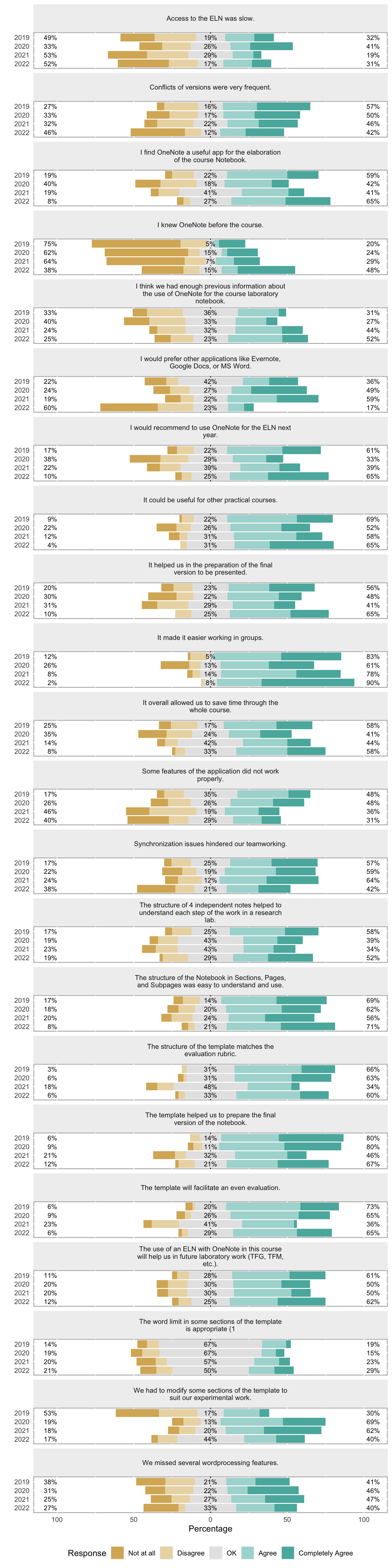
General Methodology
Course difficulty
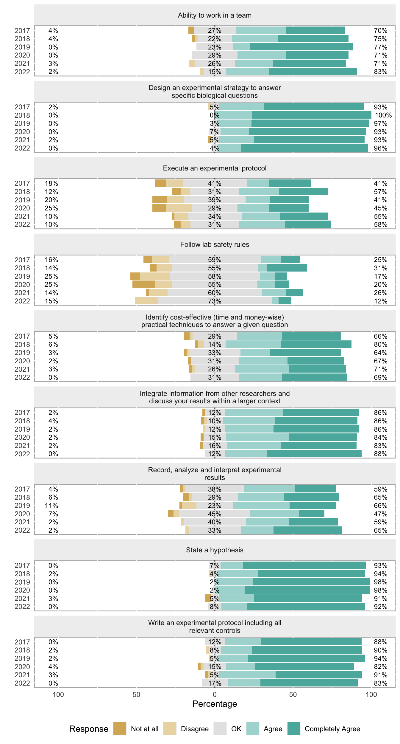
12
2017-2018
Method objectives
State a hypothesis
13
2017-2018
Method objectives
Design an experimental strategy to answer specific biological questions
14
2017-2018
Method objectives
Identify cost-effective (time and money-wise) practical techniques to answer a given question
15
2017-2018
Method objectives
Write an experimental protocol including all relevant controls
16
2017-2018
Method objectives
Execute an experimental protocol
17
2017-2018
Method objectives
Record, analyze and interpret experimental results
18
2017-2018
Method objectives
Integrate information from other researchers and discuss your results within a larger context
19
2017-2018
Method objectives
Follow lab safety rules
20
2017-2018
Method objectives
Ability to work in a team
21
2017-2018
Activities interest
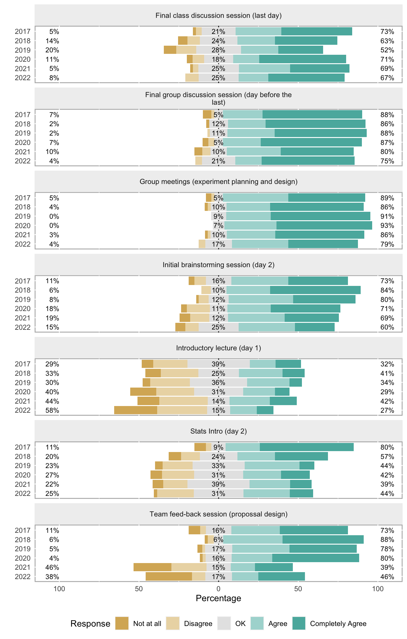
Introductory lecture (day 1)
22
2017-2018
Activities interest
Stats Intro (day 2)
23
2017-2018
Activities interest
Initial brainstorming session (day 2)
24
2017-2018
Activities interest
Group meetings (experiment planning and design)
25
2017-2018
Activities interest
Team feed-back session (propossal design)
26
2017-2018
Activities interest
Final group discussion session (day before the last)
27
2017-2018
Activities interest
Final class discussion session (last day)
28
2017-2018
Activities Length
Introductory lecture (day 1)
29
2017-2018
Activities Length
Stats Intro (day 2)
30
2017-2018
Activities Length
Initial brainstorming session (day 2)
31
2017-2018
Activities Length
Group meetings (experiment planning and design)
32
2017-2018
Activities Length
Team feed-back sessions
33
2017-2018
Activities Length
Final group discussion session (day before the last)
34
2017-2018
Activities Length
Final class discussion session (last day)
35
2017-2018
Assesment
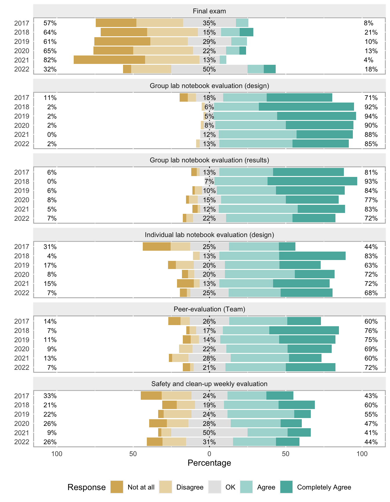
Safety and clean-up weekly evaluation
36
2017-2018
Assesment
Individual lab notebook evaluation (design)
37
2017-2018
Assesment
Group lab notebook evaluation (design)
38
2017-2018
Assesment
Group lab notebook evaluation (results)
39
2017-2018
Assesment
Peer-evaluation (Team)
40
2017-2018
Assesment
Final exam
41
2017-2018
Learning Objectives
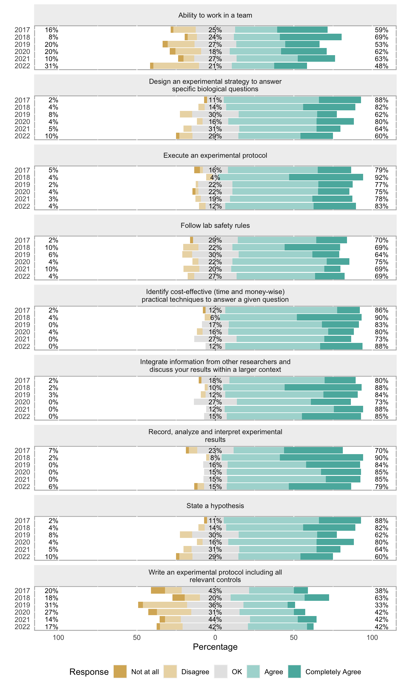
State a hypothesis
42
2017-2018
Learning Objectives
Design an experimental strategy to answer specific biological questions
43
2017-2018
Learning Objectives
Identify cost-effective (time and money-wise) practical techniques to answer a given question
44
2017-2018
Learning Objectives
Write an experimental protocol including all relevant controls
45
2017-2018
Learning Objectives
Execute an experimental protocol
46
2017-2018
Learning Objectives
Record, analyze and interpret experimental results
47
2017-2018
Learning Objectives
Integrate information from other researchers and discuss your results within a larger context
48
2017-2018
Learning Objectives
Follow lab safety rules
49
2017-2018
Learning Objectives
Ability to work in a team
50
2017-2018
Open
Best
51
2017-2018
Open
Worse
52
2017-2018
Open
Open comments
53
2019-2020
ELN
I knew OneNote before the course.
54
2019-2020
ELN
I find OneNote a useful app for the elaboration of the course Notebook.
55
2019-2020
ELN
I think we had enough previous information about the use of OneNote for the course laboratory notebook.
56
2019-2020
ELN
I would prefer other applications like Evernote, Google Docs, or MS Word.
57
2019-2020
ELN
The structure of the Notebook in Sections, Pages, and Subpages was easy to understand and use.
58
2019-2020
ELN
I would recommend to use OneNote for the ELN next year.
59
2019-2020
ELN
It overall allowed us to save time through the whole course.
60
2019-2020
ELN
It helped us in the preparation of the final version to be presented.
61
2019-2020
ELN
It made it easier working in groups.
62
2019-2020
ELN
It could be useful for other practical courses.
63
2019-2020
ELN
Synchronization issues hindered our teamworking.
64
2019-2020
ELN
Conflicts of versions were very frequent.
65
2019-2020
ELN
Access to the ELN was slow.
66
2019-2020
ELN
We missed several wordprocessing features.
67
2019-2020
ELN
Some features of the application did not work properly.
68
2019-2020
ELN
The template helped us to prepare the final version of the notebook.
69
2019-2020
ELN
The structure of the template matches the evaluation rubric.
70
2019-2020
ELN
The structure of 4 independent notes helped to understand each step of the work in a research lab.
71
2019-2020
ELN
The word limit in some sections of the template is appropriate (1
72
2019-2020
ELN
We had to modify some sections of the template to suit our experimental work.
73
2019-2020
ELN
The template will facilitate an even evaluation.
74
2019-2020
ELN
The use of an ELN with OneNote in this course will help us in future laboratory work (TFG, TFM, etc.).
75
2021-2022
Open
Open comments ELN
76
2021-2022
Open
Positive aspects about the project desing teams session
77
2021-2022
Open
Negative aspects about the project desing teams session
3 Load data and pairwise t.test
Survey responses were downloaded from Moodle as txt/csv files. Moodle updates caused some format differences that could be worked around after opening the files with Numbers and exporting them as tables with “;” as the column separator. We now show all vs. all pairwise t-tests performed to detect significant differences in responses per year. The tables below contain the pairwise p-values for each comparison, with significant values highlighted in blue (p<0.05) and red (p<0.01)
Show the code
#read the data in a list of dataframes#didn't use the headers to avoid mistakesquiz <-lapply(2017:2022, function(x) read.csv(paste0("survey",x,".csv"),header=FALSE,skip=1,sep=";"))#add Year as the third variable (empty so far)curso <-c("2017","2018","2019","2020","2021","2022")for (i in1:length(quiz)){ quiz[[i]][,3] <- curso[i]}#adjust questions changes#remove questions in column 32 & 40 from 2017, because we removed it in the following yearsquiz[[1]] <- quiz[[1]][,-c(32,40)]quiz[[6]] <- quiz[[6]][,-10]names(quiz[[6]]) <-names(quiz[[5]])names(quiz[[1]]) <-names(quiz[[2]])#merge all dataframes and name the columns data <-Reduce(function(x, y) merge(x, y, all=TRUE), quiz)#take the colnames from the last quiz that contains all the questionscolnames(data)[3] <-"Curso"#statistics analysis#subset questions 1/2: remove leftmost junk columnssubdata_all <- data[,c(3,11:87)]names(subdata_all) <-c("Curso",paste0("Q",1:77))#write.csv(subdata_all, "merged_data.csv")#subset questions 2/2: remove open questionsopen <-c(row.names(questions[questions$Section=="Open",]))subdata <- subdata_all[,-(as.integer(open)+1)]subdata <-sapply(subdata,as.numeric)subdata <-as.data.frame(subdata)#perform tests and display table in a looptests <-list()nombres <-c()for (i in2:ncol(subdata)){ subdata[,i][!(subdata[,i] %in%c(1,2,3,4,5))] <-NA#subset for years with answers to avoid void groups kkk <-subset(subdata,!is.na(subdata[,i])) tests[[i-1]] <-pairwise.t.test(x=as.numeric(kkk[,i]),g=as.numeric(kkk[,1]),paired = F) nombres[i-1] <- questions[,4][(which(questions$No. %in%gsub("\\D", "",colnames(subdata[i]))))]names(tests) <- nombresprint(as.data.frame(format(tests[[i-1]]$p.value, scientific=F,nsmall=6)) %>%replace(., . <0, "") %>%mutate_all(~cell_spec(.x, color =ifelse(.x <0.01, "firebrick", ifelse(.x <0.05, "steelblue","black")))) %>%kable(escape = F, align ="cccl", caption =paste("<b>",names(tests[i-1]),"</b>"), digits=4) %>%kable_styling(bootstrap_options ="striped", full_width = F, position ="center") %>%column_spec(1, bold = T))}
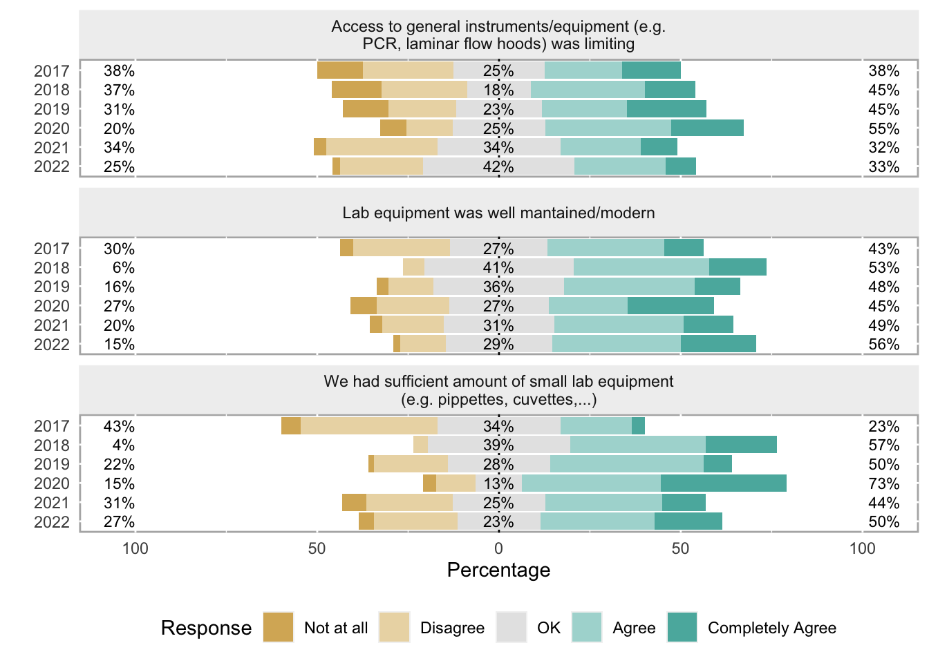
We had sufficient amount of small lab equipment (e.g. pippettes, cuvettes,…)
2017
2018
2019
2020
2021
2018
0.0000483590195
2019
0.0387917021564
0.2923742359147
2020
0.0000004884986
1.0000000000000
0.0419190959605
2021
0.2620951546148
0.0578942405845
1.0000000000000
0.0038769973311
2022
0.0419190959605
0.4547601785452
1.0000000000000
0.0921839025876
1.0000000000000
Access to general instruments/equipment (e.g. PCR, laminar flow hoods) was limiting
2017
2018
2019
2020
2021
2018
1.0000000
2019
1.0000000
1.0000000
2020
0.8109768
1.0000000
1.0000000
2021
1.0000000
1.0000000
1.0000000
0.8344372
2022
1.0000000
1.0000000
1.0000000
1.0000000
1.0000000
Lab equipment was well mantained/modern
2017
2018
2019
2020
2021
2018
0.4899485
2019
1.0000000
1.0000000
2020
1.0000000
1.0000000
1.0000000
2021
1.0000000
1.0000000
1.0000000
1.0000000
2022
0.6531043
1.0000000
1.0000000
1.0000000
1.0000000
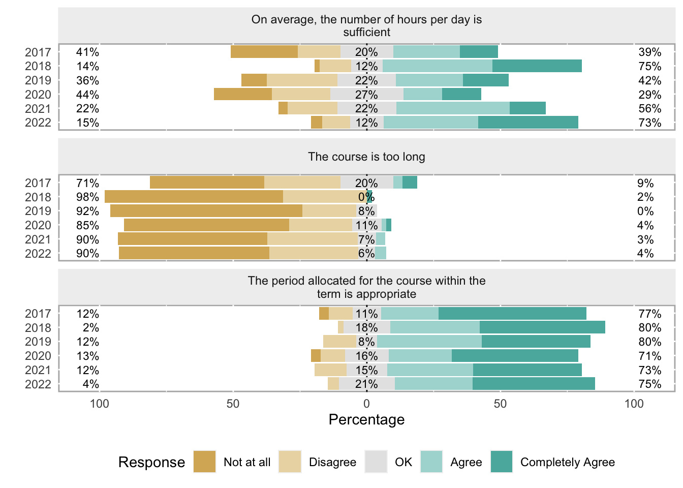
The course is too long
2017
2018
2019
2020
2021
2018
0.0026643833
2019
0.0004996605
1.0000000000
2020
0.1019667926
1.0000000000
1.0000000000
2021
0.0868213996
1.0000000000
1.0000000000
1.0000000000
2022
0.1248722514
1.0000000000
1.0000000000
1.0000000000
1.0000000000
The period allocated for the course within the term is appropriate
2017
2018
2019
2020
2021
2018
1.000000
2019
1.000000
1.000000
2020
1.000000
1.000000
1.000000
2021
1.000000
1.000000
1.000000
1.000000
2022
1.000000
1.000000
1.000000
1.000000
1.000000
On average, the number of hours per day is sufficient
2017
2018
2019
2020
2021
2018
0.00017408424
2019
0.70836310750
0.00827853160
2020
1.00000000000
0.00003732550
0.55774777454
2021
0.10939218514
0.28372061782
0.69993349604
0.03884955505
2022
0.00023825512
1.00000000000
0.00991069098
0.00005433618
0.28372061782
Student engagement
2017
2018
2019
2020
2021
2018
1.0000000
2019
1.0000000
1.0000000
2020
1.0000000
0.2189352
0.3199053
2021
1.0000000
1.0000000
1.0000000
1.0000000
2022
1.0000000
1.0000000
1.0000000
0.1269859
1.0000000
Course interest
2017
2018
2019
2020
2021
2018
1.0000000
2019
1.0000000
1.0000000
2020
0.2988613
1.0000000
1.0000000
2021
1.0000000
1.0000000
1.0000000
0.1231708
2022
1.0000000
1.0000000
1.0000000
0.3158588
1.0000000
Course usefulness
2017
2018
2019
2020
2021
2018
1.0000000
2019
1.0000000
1.0000000
2020
1.0000000
0.3070813
0.4019150
2021
1.0000000
1.0000000
1.0000000
0.2706641
2022
1.0000000
1.0000000
1.0000000
1.0000000
1.0000000
Demand on student’s part
2017
2018
2019
2020
2021
2018
1.000000
2019
1.000000
1.000000
2020
1.000000
1.000000
1.000000
2021
1.000000
1.000000
1.000000
1.000000
2022
1.000000
1.000000
1.000000
1.000000
1.000000
Course difficulty
2017
2018
2019
2020
2021
2018
1.00000000
2019
1.00000000
1.00000000
2020
0.59959609
0.20871738
0.75236097
2021
1.00000000
1.00000000
1.00000000
1.00000000
2022
1.00000000
1.00000000
1.00000000
0.09488378
1.00000000
State a hypothesis
2017
2018
2019
2020
2021
2018
1.0000000
2019
1.0000000
1.0000000
2020
1.0000000
1.0000000
1.0000000
2021
1.0000000
1.0000000
1.0000000
0.5792492
2022
1.0000000
1.0000000
1.0000000
1.0000000
1.0000000
Design an experimental strategy to answer specific biological questions
2017
2018
2019
2020
2021
2018
0.9819431
2019
1.0000000
1.0000000
2020
1.0000000
1.0000000
1.0000000
2021
1.0000000
1.0000000
1.0000000
1.0000000
2022
0.9819431
1.0000000
1.0000000
1.0000000
1.0000000
Identify cost-effective (time and money-wise) practical techniques to answer a given question
2017
2018
2019
2020
2021
2018
1.000000
2019
1.000000
1.000000
2020
1.000000
1.000000
1.000000
2021
1.000000
1.000000
1.000000
1.000000
2022
1.000000
1.000000
1.000000
1.000000
1.000000
Write an experimental protocol including all relevant controls
2017
2018
2019
2020
2021
2018
1.0000000
2019
1.0000000
1.0000000
2020
1.0000000
1.0000000
0.8385782
2021
1.0000000
1.0000000
0.9188235
1.0000000
2022
1.0000000
1.0000000
1.0000000
1.0000000
1.0000000
Execute an experimental protocol
2017
2018
2019
2020
2021
2018
1.000000
2019
1.000000
1.000000
2020
1.000000
1.000000
1.000000
2021
1.000000
1.000000
1.000000
1.000000
2022
1.000000
1.000000
1.000000
1.000000
1.000000
Record, analyze and interpret experimental results
2017
2018
2019
2020
2021
2018
1.00000000
2019
1.00000000
1.00000000
2020
1.00000000
0.63038271
1.00000000
2021
1.00000000
1.00000000
1.00000000
0.67234486
2022
1.00000000
1.00000000
1.00000000
0.07443221
1.00000000
Integrate information from other researchers and discuss your results within a larger context
2017
2018
2019
2020
2021
2018
1.000000
2019
1.000000
1.000000
2020
1.000000
1.000000
1.000000
2021
1.000000
1.000000
1.000000
1.000000
2022
1.000000
1.000000
1.000000
1.000000
1.000000
Follow lab safety rules
2017
2018
2019
2020
2021
2018
1.0000000
2019
1.0000000
0.1591204
2020
1.0000000
0.1062739
1.0000000
2021
1.0000000
1.0000000
1.0000000
1.0000000
2022
1.0000000
1.0000000
1.0000000
1.0000000
1.0000000
Ability to work in a team
2017
2018
2019
2020
2021
2018
1.0000000
2019
0.1609205
1.0000000
2020
1.0000000
1.0000000
0.7693568
2021
1.0000000
1.0000000
0.9866925
1.0000000
2022
0.4842893
1.0000000
1.0000000
1.0000000
1.0000000
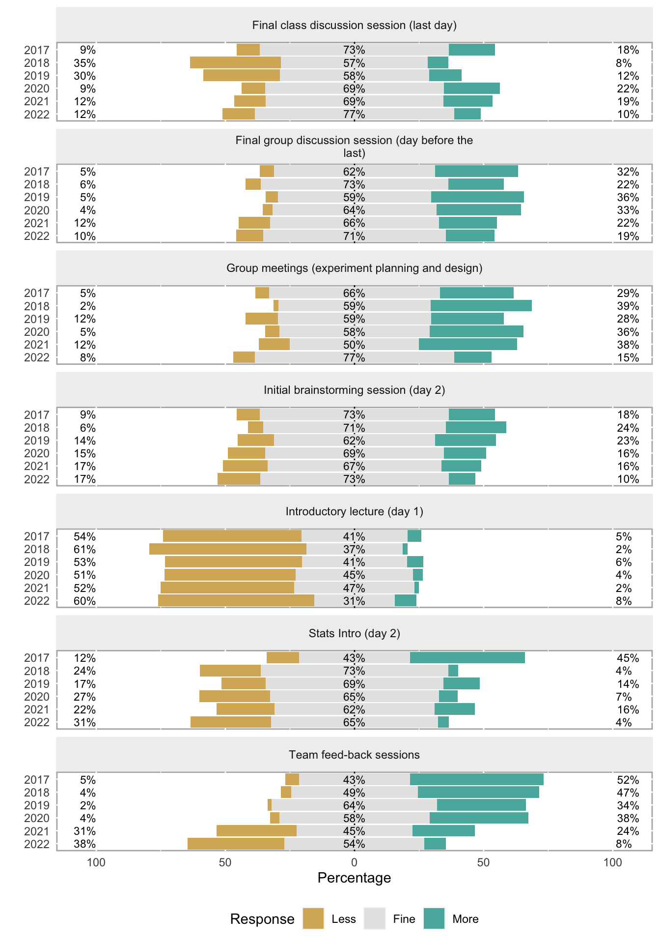
Introductory lecture (day 1)
2017
2018
2019
2020
2021
2018
1.0000000
2019
1.0000000
1.0000000
2020
1.0000000
1.0000000
1.0000000
2021
1.0000000
1.0000000
1.0000000
1.0000000
2022
0.1719199
0.2035414
0.2110407
1.0000000
0.4244263
Stats Intro (day 2)
2017
2018
2019
2020
2021
2018
0.09016649012
2019
0.00008152269
0.74311961810
2020
0.00016320717
0.74650659356
1.00000000000
2021
0.00008674063
0.74311961810
1.00000000000
1.00000000000
2022
0.00085888056
1.00000000000
1.00000000000
1.00000000000
1.00000000000
Initial brainstorming session (day 2)
2017
2018
2019
2020
2021
2018
0.73502136
2019
1.00000000
1.00000000
2020
1.00000000
0.54883014
1.00000000
2021
1.00000000
0.08910869
1.00000000
1.00000000
2022
1.00000000
0.02113266
0.42132644
1.00000000
1.00000000
Group meetings (experiment planning and design)
2017
2018
2019
2020
2021
2018
1.0000000
2019
1.0000000
1.0000000
2020
1.0000000
1.0000000
1.0000000
2021
1.0000000
1.0000000
1.0000000
1.0000000
2022
1.0000000
1.0000000
0.4134602
0.4928046
1.0000000
Team feed-back session (propossal design)
2017
2018
2019
2020
2021
2018
1.00000000000000
2019
1.00000000000000
1.00000000000000
2020
1.00000000000000
1.00000000000000
1.00000000000000
2021
0.00005122068635
0.00000009484981
0.00000132369981
0.00000009133855
2022
0.00158018907055
0.00000922139896
0.00008708905906
0.00000922139896
1.00000000000000
Final group discussion session (day before the last)
2017
2018
2019
2020
2021
2018
1.0000000
2019
1.0000000
1.0000000
2020
1.0000000
1.0000000
1.0000000
2021
1.0000000
0.8147184
0.8058628
1.0000000
2022
1.0000000
1.0000000
1.0000000
1.0000000
1.0000000
Final class discussion session (last day)
2017
2018
2019
2020
2021
2018
1.00000000
2019
0.05752352
1.00000000
2020
1.00000000
1.00000000
0.05752352
2021
1.00000000
1.00000000
0.19394869
1.00000000
2022
1.00000000
1.00000000
0.13401895
1.00000000
1.00000000
Introductory lecture (day 1)
2017
2018
2019
2020
2021
2018
1.000000
2019
1.000000
1.000000
2020
1.000000
1.000000
1.000000
2021
1.000000
1.000000
1.000000
1.000000
2022
1.000000
1.000000
1.000000
1.000000
1.000000
Stats Intro (day 2)
2017
2018
2019
2020
2021
2018
0.000079202174
2019
0.011210736317
0.923397980687
2020
0.000048127766
1.000000000000
0.923189334071
2021
0.004677895906
1.000000000000
1.000000000000
1.000000000000
2022
0.000005872309
1.000000000000
0.316437132574
1.000000000000
0.684925357179
Initial brainstorming session (day 2)
2017
2018
2019
2020
2021
2018
1.0000000
2019
1.0000000
1.0000000
2020
1.0000000
1.0000000
1.0000000
2021
1.0000000
0.9746626
1.0000000
1.0000000
2022
1.0000000
0.4920238
1.0000000
1.0000000
1.0000000
Group meetings (experiment planning and design)
2017
2018
2019
2020
2021
2018
1.0000000
2019
1.0000000
0.5996380
2020
1.0000000
1.0000000
1.0000000
2021
1.0000000
1.0000000
1.0000000
1.0000000
2022
1.0000000
0.1165861
1.0000000
0.4314979
0.9808853
Team feed-back sessions
2017
2018
2019
2020
2021
2018
1.000000000000000
2019
1.000000000000000
1.000000000000000
2020
1.000000000000000
1.000000000000000
1.000000000000000
2021
0.000038830019899
0.000206638825759
0.002745649027283
0.002745649027283
2022
0.000000009589759
0.000000091479031
0.000001842477928
0.000002020658358
0.415623067641416
Final group discussion session (day before the last)
2017
2018
2019
2020
2021
2018
1.0000000
2019
1.0000000
1.0000000
2020
1.0000000
1.0000000
1.0000000
2021
1.0000000
1.0000000
0.5053068
0.8400922
2022
0.9660558
1.0000000
0.4379554
0.7278093
1.0000000
Final class discussion session (last day)
2017
2018
2019
2020
2021
2018
0.01265194
2019
0.12572353
1.00000000
2020
1.00000000
0.00403720
0.04786672
2021
1.00000000
0.02036425
0.18483993
1.00000000
2022
1.00000000
0.22708031
1.00000000
1.00000000
1.00000000
Safety and clean-up weekly evaluation
2017
2018
2019
2020
2021
2018
1.000000
2019
1.000000
1.000000
2020
1.000000
1.000000
1.000000
2021
1.000000
1.000000
1.000000
1.000000
2022
1.000000
1.000000
1.000000
1.000000
1.000000
Individual lab notebook evaluation (design)
2017
2018
2019
2020
2021
2018
0.000005986044
2019
0.036241990530
0.151546760594
2020
0.003708188789
0.962130275199
1.000000000000
2021
0.004132922998
0.803268104984
1.000000000000
1.000000000000
2022
0.002823163299
1.000000000000
1.000000000000
1.000000000000
1.000000000000
Group lab notebook evaluation (design)
2017
2018
2019
2020
2021
2018
0.009839814
2019
0.030480248
1.000000000
2020
0.326865132
1.000000000
1.000000000
2021
0.862805649
0.862805649
1.000000000
1.000000000
2022
1.000000000
0.582027990
1.000000000
1.000000000
1.000000000
Group lab notebook evaluation (results)
2017
2018
2019
2020
2021
2018
0.77614926
2019
1.00000000
0.85014326
2020
1.00000000
0.08987183
1.00000000
2021
1.00000000
0.11606382
1.00000000
1.00000000
2022
1.00000000
0.02078403
0.93011672
1.00000000
1.00000000
Peer-evaluation (Team)
2017
2018
2019
2020
2021
2018
0.2010087
2019
0.9374738
1.0000000
2020
1.0000000
1.0000000
1.0000000
2021
1.0000000
0.4252861
1.0000000
1.0000000
2022
1.0000000
1.0000000
1.0000000
1.0000000
1.0000000
Final exam
2017
2018
2019
2020
2021
2018
1.00000000000
2019
1.00000000000
1.00000000000
2020
1.00000000000
1.00000000000
1.00000000000
2021
0.19443594677
0.11192572029
0.58882936651
0.19443594677
2022
0.04751643983
0.24253304906
0.00806879380
0.06184887152
0.00001291026
State a hypothesis
2017
2018
2019
2020
2021
2018
1.00000000
2019
0.04850727
0.04850727
2020
1.00000000
1.00000000
0.24054592
2021
0.17406452
0.17406452
1.00000000
0.64176390
2022
0.10429512
0.10429512
1.00000000
0.39469018
1.00000000
Design an experimental strategy to answer specific biological questions
2017
2018
2019
2020
2021
2018
0.22569250
2019
1.00000000
1.00000000
2020
1.00000000
0.11316070
1.00000000
2021
1.00000000
0.05348894
1.00000000
1.00000000
2022
1.00000000
1.00000000
1.00000000
1.00000000
0.69996632
Identify cost-effective (time and money-wise) practical techniques to answer a given question
2017
2018
2019
2020
2021
2018
0.8223218
2019
1.0000000
0.1174194
2020
1.0000000
0.8007973
1.0000000
2021
1.0000000
1.0000000
0.8007973
1.0000000
2022
1.0000000
1.0000000
1.0000000
1.0000000
1.0000000
Write an experimental protocol including all relevant controls
2017
2018
2019
2020
2021
2018
0.05017013
2019
1.00000000
0.11678843
2020
1.00000000
0.03687698
1.00000000
2021
1.00000000
0.22014254
1.00000000
1.00000000
2022
1.00000000
0.71000111
1.00000000
1.00000000
1.00000000
Execute an experimental protocol
2017
2018
2019
2020
2021
2018
0.06715688
2019
1.00000000
1.00000000
2020
1.00000000
0.59128042
1.00000000
2021
1.00000000
0.29344923
1.00000000
1.00000000
2022
1.00000000
0.59277265
1.00000000
1.00000000
1.00000000
Record, analyze and interpret experimental results
2017
2018
2019
2020
2021
2018
0.05965194
2019
1.00000000
0.17943892
2020
1.00000000
0.08604197
1.00000000
2021
1.00000000
0.38331922
1.00000000
1.00000000
2022
0.57856745
1.00000000
1.00000000
0.71376191
1.00000000
Integrate information from other researchers and discuss your results within a larger context
2017
2018
2019
2020
2021
2018
1.000000
2019
1.000000
1.000000
2020
1.000000
1.000000
1.000000
2021
1.000000
1.000000
1.000000
1.000000
2022
1.000000
1.000000
1.000000
1.000000
1.000000
Follow lab safety rules
2017
2018
2019
2020
2021
2018
1.0000000
2019
1.0000000
0.3584685
2020
1.0000000
1.0000000
1.0000000
2021
1.0000000
1.0000000
1.0000000
1.0000000
2022
1.0000000
0.0763971
1.0000000
1.0000000
1.0000000
Ability to work in a team
2017
2018
2019
2020
2021
2018
0.5300693
2019
1.0000000
1.0000000
2020
1.0000000
0.9486344
1.0000000
2021
1.0000000
1.0000000
1.0000000
1.0000000
2022
1.0000000
1.0000000
1.0000000
1.0000000
1.0000000
I knew OneNote before the course.
2019
2020
2021
2020
1.000000000
2021
1.000000000
1.000000000
2022
0.001084163
0.016734935
0.016734935
I find OneNote a useful app for the elaboration of the course Notebook.
2019
2020
2021
2020
0.0194452005
2021
0.4290317085
0.4290317085
2022
0.4290317085
0.0009279188
0.0533435476
I think we had enough previous information about the use of OneNote for the course laboratory notebook.
2019
2020
2021
2020
0.90321465
2021
0.26475274
0.08479041
2022
0.26475274
0.08179045
0.90321465
I would prefer other applications like Evernote, Google Docs, or MS Word.
2019
2020
2021
2020
0.350094297658
2021
0.285699438100
0.780655259274
2022
0.000694996965
0.000007056524
0.000001613306
The structure of the Notebook in Sections, Pages, and Subpages was easy to understand and use.
2019
2020
2021
2020
1.0000000
2021
1.0000000
1.0000000
2022
1.0000000
0.9442328
0.9442328
I would recommend to use OneNote for the ELN next year.
2019
2020
2021
2020
0.00221548731
2021
0.17292060827
0.19622364895
2022
0.22861804207
0.00006958609
0.01373391161
It overall allowed us to save time through the whole course.
2019
2020
2021
2020
0.30524952
2021
0.71580658
0.54233771
2022
0.55642049
0.03337407
0.54233771
It helped us in the preparation of the final version to be presented.
2019
2020
2021
2020
0.17015091
2021
0.17015091
0.95581757
2022
0.70626759
0.03746040
0.03256321
It made it easier working in groups.
2019
2020
2021
2020
0.01181063530
2021
0.50976729000
0.05372194665
2022
0.10713884537
0.00002366656
0.04984516896
It could be useful for other practical courses.
2019
2020
2021
2020
0.096914036
2021
0.559296396
0.598200546
2022
0.598200546
0.009901279
0.103501098
Synchronization issues hindered our teamworking.
2019
2020
2021
2020
1.00000000
2021
1.00000000
1.00000000
2022
0.06488059
0.23221748
0.06488059
Conflicts of versions were very frequent.
2019
2020
2021
2020
0.74604855
2021
0.74604855
0.97106146
2022
0.03894251
0.52018190
0.52018190
Access to the ELN was slow.
2019
2020
2021
2020
0.23259370
2021
0.78929605
0.02082084
2022
1.00000000
0.10289719
1.00000000
We missed several wordprocessing features.
2019
2020
2021
2020
1.000000
2021
1.000000
1.000000
2022
1.000000
1.000000
1.000000
Some features of the application did not work properly.
2019
2020
2021
2020
1.00000000
2021
0.11460584
0.19561512
2022
0.05474198
0.11460584
1.00000000
The template helped us to prepare the final version of the notebook.
2019
2020
2021
2020
0.76183109293
2021
0.00001688823
0.00040185259
2022
0.39992415566
0.76183109293
0.01161284601
The structure of the template matches the evaluation rubric.
2019
2020
2021
2020
1.0000000000
2021
0.0001986663
0.0009679592
2022
1.0000000000
1.0000000000
0.0067090936
The structure of 4 independent notes helped to understand each step of the work in a research lab.
2019
2020
2021
2020
0.7663575
2021
0.2501597
0.9376949
2022
0.9376949
0.7663575
0.2501597
The word limit in some sections of the template is appropriate (1
2019
2020
2021
2020
1.000000
2021
1.000000
1.000000
2022
1.000000
1.000000
1.000000
We had to modify some sections of the template to suit our experimental work.
2019
2020
2021
2020
0.000003220546
2021
0.000001115448
0.842569147842
2022
0.001868462978
0.359412324506
0.359412324506
The template will facilitate an even evaluation.
2019
2020
2021
2020
0.99796751647
2021
0.00006709339
0.00350600194
2022
1.00000000000
1.00000000000
0.00117637850
The use of an ELN with OneNote in this course will help us in future laboratory work (TFG, TFM, etc.).
2019
2020
2021
2020
0.4321188
2021
0.4232123
1.0000000
2022
1.0000000
0.4232123
0.3318217
4 Likert scale plots
Likert scale responses are grouped by the sections in the quiz.
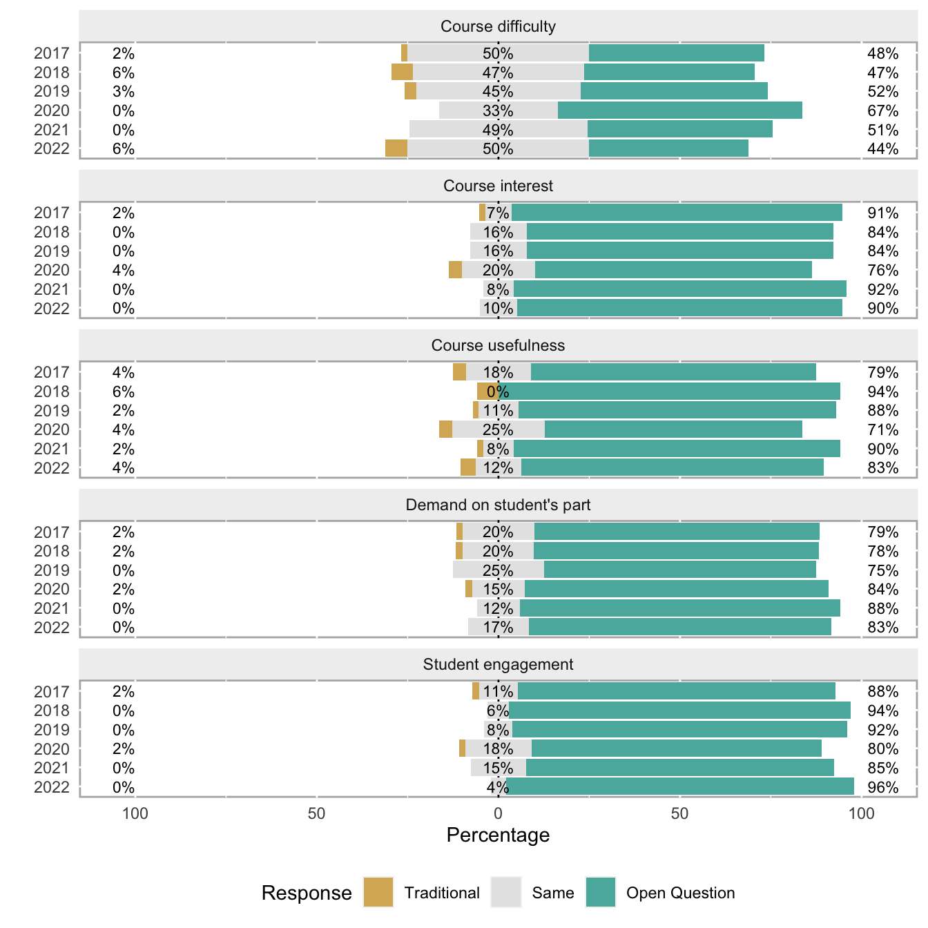
4.1 General Methodology
Show the code
#lickert#change question namestablita <-data.frame(matrix(NA, # Create empty data framenrow =length(colnames(subdata)),ncol =2))for (i in2:length(colnames(subdata))){ tablita[i-1,] <-cbind(colnames(subdata[i]),questions$Question[as.numeric(gsub("\\D", "",colnames(subdata[i])))])colnames(subdata)[i] <- tablita[i-1,2]}for (i in2:72){ subdata[,i] <-factor(subdata[,i])}subdata$Curso <-factor(subdata$Curso,levels=c(2022,2021,2020,2019,2018,2017))#questions with 3 options#General Methodologysubdata[,c(8:12)] <-lapply(subdata[,c(8:12)], function(x) factor(x, labels =c("Traditional","Same","Open Question")) )xlikgroup3a =likert(subdata[,c(8:12)], grouping = subdata$Curso)plot(xlikgroup3a, type ="bar", centered = T)