R3: Read and write data in R

Input

Output

Read

Write

Path

Working Directory

Published

May 30, 2023

Modified

November 22, 2023

1 Data input & output in R

As you already know, launching R starts an interactive session with input from the keyboard and output on the screen. If you are using small datasets, you can define and enter your data directly in the Console, as you did in the examples before. Also, you can define your objects and enter your data interactively with the functions scan() and readline() as in the examples below. Regarding the output, you can just call the object by its name or use the function print(), which displays on the screen the contents of its argument object. You can try the code below.¹

vector <- scan(n = 4)
vector2 <- scan()
str <- readline()
vector
print(vector2)
print(str)
edit(str)

Although, seldom used, you can also edit the contents of your objects using the function edit(). This function can be used to edit different objects, including vectors, strings, matrices or dataframes. MacOS users may need to install XQuartz X11 tool.

2 Working directory

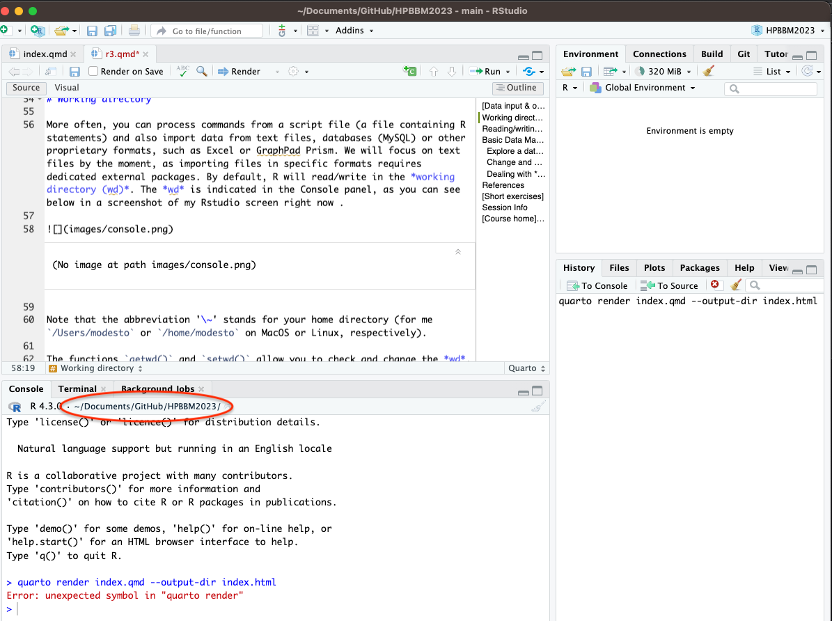
More often, you can process commands from a script file (a file containing R statements) and also import data from text files, databases (MySQL) or other proprietary formats, such as Excel or GraphPad Prism. We will focus on text files by the moment, as importing files in specific formats requires dedicated external packages. By default, R will read/write in the working directory (wd). The wd is indicated in the Console panel, as you can see below in a screenshot of my Rstudio screen right now.

Note that the abbreviation ‘~’ stands for your home directory (for me /Users/modesto or /home/modesto on MacOS or Linux, respectively).

The functions getwd() and setwd() allow you to check and change the wd. Try the examples below and pay attention to the output. Remember that you can write ?getwd() or ?setwd() for help.

getwd()

[1] "/Users/modesto/Documents/GitHub/HPBBM2023"

setwd("/Users/modesto")
getwd()

[1] "/Users/modesto"

# Obviously the path must call an existing directory (no
# typos allowed)
setwd("/Users/modsto/Documents/GitHub/HPBBM2023")

Error in setwd("/Users/modsto/Documents/GitHub/HPBBM2023"): cannot change working directory

setwd("/Users/modesto/Documents/GitHub/HPBBM2023")
getwd()

[1] "/Users/modesto/Documents/GitHub/HPBBM2023"

In RStudio, the default working directory can be set from the “tools” and “global options” menu. Also, you can change the wd for your session in the menu Session > Set Working Directory and change it to that of source file (for instant your R script), the project or the selected directory in the files panel.

2.1 Quick exercise (I)

Let’s see if you understood. Consider the following tree of directories.

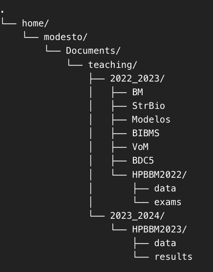
How would you change de wd to the folder HPBBM2023/data? You also can try with your own computer and your directory tree.

Select the right answer

setwd(“HPBBM2023/data”) setwd(“/home/modesto/Documents/teaching/2023_2024/HPBBM2023/data”) setwd(“/Users/modesto/teaching/Documents/2023_2024/HPBBM2023/data”)

3 Reading/writing data in R

The most common way to read your data in R is importing it as a table, using the function read.table(). Note that the resultant object will become a Dataframe, even when all the entries got to be numeric. A followup call towards as.matrix() will turn it into in a matrix.

In the following example lines we read a file called small_matrix.csv, located in the data folder. If we attempt to make some matrix calculations, R will force the dataframe to a matrix when possible, but it will return an Error for many matrix-specific operations or functions unless, we transform the dataframe into a matrix.

sm <- read.table("small_matrix.csv", sep = ",")  #what happens here?

Warning in file(file, "rt"): cannot open file 'small_matrix.csv': No such file
or directory

Error in file(file, "rt"): cannot open the connection

# check the path
getwd()

[1] "/Users/modesto/Documents/GitHub/HPBBM2023"

# now we use the right path
sm <- read.table("data/small_matrix.csv", sep = ",")
sm

# is this an object type matrix?
is.matrix(sm)

[1] FALSE

# can we operate with it as a matrix?
t(sm)

   [,1] [,2] [,3] [,4]
V1    2   22   18   25
V2    7   10    3    6
V3   19   80   13   16

# we can force an object to operate as a matrix
sm * 3

  V1 V2  V3
1  6 21  57
2 66 30 240
3 54  9  39
4 75 18  48

diag(sm)

Error in diag(sm): 'list' object cannot be coerced to type 'double'

# some operations cannot coerce a matrix but we can
# explicit it
diag(as.matrix(sm))

[1]  2 10 13

heatmap(sm)

Error in heatmap(sm): 'x' must be a numeric matrix

heatmap(as.matrix(sm))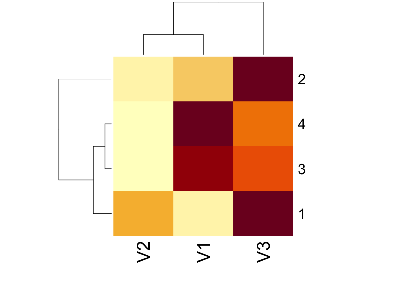

Tip

Note that read.table() and its wrappers read.csv() or read.csv2() are mostly use for reading dataframes. If your want to read text files, like in the case of biological sequences, you can use other functions, like readLines(), described in the Lesson 9.

You can write any data object(s) as binary data file or as text files. Compare the different files saved in the code below.

vector <- c(1:5)
vector2 <- c(3, 5:13)
write(vector2, file = "data/vector2.txt")
write.table(sm, "data/sm.csv")
write.table(sm, "data/sm2.csv", row.names = FALSE, col.names = FALSE,
    sep = ",")

save(vector, vector2, file = "data/vector2.Rdata")
save.image(file = "data/myEnvironment.RData")

Data files in RData format can be open from the Environment tab or with the load() function. To check that it was correctly loaded, we can remove it before loading with the rm() function.

# remove from the Global Environment in our RStudio session
rm(vector)
rm(vector2)
# load again
load("data/vector2.Rdata")
vector

[1] 1 2 3 4 5

vector2

 [1]  3  5  6  7  8  9 10 11 12 13

Caution

Note that if you save your data with save(), it cannot be restored under a different name. The original object names are automatically used. If you want to save the object and restore it with a different name you need to use the functions saveRDS() and readRDS()

3.1 Quick exercise (II)

We are using the same directory tree. Your wd is HPBBM2022/data and you need to save a data.frame named table1 as table1.csv in the folder HPBBM2023/data using ; as separator. How would you do it without changing the working directory? Try it also with your own computer.

Select the right answer

write.table(table1, “../../../HPBBM2023/data/table1.csv”, sep=“;”) write.table(table1, “../../HPBBM2023/data/table1.csv”, sep=“;”) write.table(table1, “../../../HPBBM2023/data/table1.csv”)

4 Basic Data Management in R

Now we are going to import and explore an example dataset, containing metadata from an Illumina sequencing project of pathogenic E. coli strains (Flament-Simon et al. 2020, https://doi.org/10.1038/s41598-020-69356-6). However, for didactic purposes, the original data have been simplified and manipulated and the attached datasets do not fully correspond to the actual data.

4.1 Open and explore a dataframe

As you can see in the R help, the function read.table() has several default options as FALSE, like header=FALSE. When you have a spreadsheet export file, i.e. having a table where the fields are divided by commas in place of spaces, you can use read.csv() in place of read.table(). For Spaniards, there is also read.csv2(), which uses a comma for the decimal point and a semicolon for the separator. The latter functions are wrappers of read.table() with custom default options. Likewise, there are write.csv() and write.csv2(), which are wrappers of write.table(). Look carefully at the following examples of different ways to open a table (with some common mistakes) and explore them quickly.

# Note differences between read.table(), read.csv() and
# read.csv2()
coli_genomes <- read.table(file = "data/coli_genomes.csv")

Error in scan(file = file, what = what, sep = sep, quote = quote, dec = dec, : line 2 did not have 11 elements

head(coli_genomes)

Error in eval(expr, envir, enclos): object 'coli_genomes' not found

coli_genomes <- read.table(file = "data/coli_genomes.csv", sep = ";",
    dec = ".", header = TRUE)
head(coli_genomes)

   Strain    Biosample Year.of.isolation   Source Phylogroup Serotype Clonotype
1 LREC237 SAMN14278613                NA   Human           D  ONT:H28  CH23-331
2 LREC239 SAMN14278614              2010   Human           C O153:H19    CH4-25
3 LREC240 SAMN14278615              2008   Human          B1  O76:H30   CH29-38
4 LREC241 SAMN14278616                NA    Human          A  O78:H11   CH11-41
5 LREC242 SAMN14278617              2011 Porcine           A  ONT:HNM    CH7-54
6 LREC243 SAMN14278618              2007 Porcine           A   O9:H37    CH7-31
  Sequence.Type VF No..Plasmids kmer Contigs    N50 longest.contig..bp.
1         ST524 18            3  117     223 272287              662555
2          ST88 14            3  117     159 323172              760527
3         ST156 10            2   89     114 270767              738861
4          ST48  5            3  117     212 112160              285056
5         ST746  5            9   89     320  45936              128053
6        ST3011  7            3   93     158 106897              369508
  total.assembled.bp contigs...1kb
1            5341632            74
2            5415613            57
3            4875343            47
4            5167401           101
5            4858138           212
6            4638334            93

coli_genomes <- read.csv(file = "data/coli_genomes.csv")
head(coli_genomes)

  Strain.Biosample.Year.of.isolation.Source.Phylogroup.Serotype.Clonotype.Sequence.Type.VF.No..Plasmids.kmer.Contigs.N50.longest.contig..bp..total.assembled.bp.contigs...1kb
1                                                                               LREC237;SAMN14278613;NA;Human ;D;ONT:H28;CH23-331;ST524;18;3;117;223;272287;662555;5341632;74
2                                                                               LREC239;SAMN14278614;2010;Human ;C;O153:H19;CH4-25;ST88;14;3;117;159;323172;760527;5415613;57
3                                                                              LREC240;SAMN14278615;2008;Human ;B1;O76:H30;CH29-38;ST156;10;2;89;114;270767;738861;4875343;47
4                                                                                  LREC241;SAMN14278616;NA;Human;A;O78:H11;CH11-41;ST48;5;3;117;212;112160;285056;5167401;101
5                                                                               LREC242;SAMN14278617;2011;Porcine ;A;ONT:HNM;CH7-54;ST746;5;9;89;320;45936;128053;4858138;212
6                                                                               LREC243;SAMN14278618;2007;Porcine ;A;O9:H37;CH7-31;ST3011;7;3;93;158;106897;369508;4638334;93

coli_genomes <- read.csv(file = "data/coli_genomes.csv", sep = ";")
head(coli_genomes)

   Strain    Biosample Year.of.isolation   Source Phylogroup Serotype Clonotype
1 LREC237 SAMN14278613                NA   Human           D  ONT:H28  CH23-331
2 LREC239 SAMN14278614              2010   Human           C O153:H19    CH4-25
3 LREC240 SAMN14278615              2008   Human          B1  O76:H30   CH29-38
4 LREC241 SAMN14278616                NA    Human          A  O78:H11   CH11-41
5 LREC242 SAMN14278617              2011 Porcine           A  ONT:HNM    CH7-54
6 LREC243 SAMN14278618              2007 Porcine           A   O9:H37    CH7-31
  Sequence.Type VF No..Plasmids kmer Contigs    N50 longest.contig..bp.
1         ST524 18            3  117     223 272287              662555
2          ST88 14            3  117     159 323172              760527
3         ST156 10            2   89     114 270767              738861
4          ST48  5            3  117     212 112160              285056
5         ST746  5            9   89     320  45936              128053
6        ST3011  7            3   93     158 106897              369508
  total.assembled.bp contigs...1kb
1            5341632            74
2            5415613            57
3            4875343            47
4            5167401           101
5            4858138           212
6            4638334            93

coli_genomes <- read.csv2(file = "data/coli_genomes.csv")
head(coli_genomes)

   Strain    Biosample Year.of.isolation   Source Phylogroup Serotype Clonotype
1 LREC237 SAMN14278613                NA   Human           D  ONT:H28  CH23-331
2 LREC239 SAMN14278614              2010   Human           C O153:H19    CH4-25
3 LREC240 SAMN14278615              2008   Human          B1  O76:H30   CH29-38
4 LREC241 SAMN14278616                NA    Human          A  O78:H11   CH11-41
5 LREC242 SAMN14278617              2011 Porcine           A  ONT:HNM    CH7-54
6 LREC243 SAMN14278618              2007 Porcine           A   O9:H37    CH7-31
  Sequence.Type VF No..Plasmids kmer Contigs    N50 longest.contig..bp.
1         ST524 18            3  117     223 272287              662555
2          ST88 14            3  117     159 323172              760527
3         ST156 10            2   89     114 270767              738861
4          ST48  5            3  117     212 112160              285056
5         ST746  5            9   89     320  45936              128053
6        ST3011  7            3   93     158 106897              369508
  total.assembled.bp contigs...1kb
1            5341632            74
2            5415613            57
3            4875343            47
4            5167401           101
5            4858138           212
6            4638334            93

# read some data
head(coli_genomes)

   Strain    Biosample Year.of.isolation   Source Phylogroup Serotype Clonotype
1 LREC237 SAMN14278613                NA   Human           D  ONT:H28  CH23-331
2 LREC239 SAMN14278614              2010   Human           C O153:H19    CH4-25
3 LREC240 SAMN14278615              2008   Human          B1  O76:H30   CH29-38
4 LREC241 SAMN14278616                NA    Human          A  O78:H11   CH11-41
5 LREC242 SAMN14278617              2011 Porcine           A  ONT:HNM    CH7-54
6 LREC243 SAMN14278618              2007 Porcine           A   O9:H37    CH7-31
  Sequence.Type VF No..Plasmids kmer Contigs    N50 longest.contig..bp.
1         ST524 18            3  117     223 272287              662555
2          ST88 14            3  117     159 323172              760527
3         ST156 10            2   89     114 270767              738861
4          ST48  5            3  117     212 112160              285056
5         ST746  5            9   89     320  45936              128053
6        ST3011  7            3   93     158 106897              369508
  total.assembled.bp contigs...1kb
1            5341632            74
2            5415613            57
3            4875343            47
4            5167401           101
5            4858138           212
6            4638334            93

tail(coli_genomes, n = 2)

    Strain    Biosample Year.of.isolation Source Phylogroup Serotype Clonotype
24 LREC261 SAMN14278636              2016 Human           A  O98:H26   CH27-23
25 LREC262 SAMN14278637              2012 Human          B1  O66:H10    CH4-32
   Sequence.Type VF No..Plasmids kmer Contigs    N50 longest.contig..bp.
24        ST8233  2            4   89     114 187945              537848
25        ST1049  4            2  113      94 325747              822206
   total.assembled.bp contigs...1kb
24            4821342            53
25            4839344            32

coli_genomes[1, ]

   Strain    Biosample Year.of.isolation Source Phylogroup Serotype Clonotype
1 LREC237 SAMN14278613                NA Human           D  ONT:H28  CH23-331
  Sequence.Type VF No..Plasmids kmer Contigs    N50 longest.contig..bp.
1         ST524 18            3  117     223 272287              662555
  total.assembled.bp contigs...1kb
1            5341632            74

coli_genomes[, 1]

 [1] "LREC237" "LREC239" "LREC240" "LREC241" "LREC242" "LREC243" "LREC244"
 [8] "LREC245" "LREC246" "LREC247" "LREC248" "LREC249" "LREC250" "LREC251"
[15] "LREC252" "LREC253" "LREC254" "LREC255" "LREC256" "LREC257" "LREC258"
[22] "LREC259" "LREC260" "LREC261" "LREC262"

coli_genomes[1:6, 2:4]

     Biosample Year.of.isolation   Source
1 SAMN14278613                NA   Human 
2 SAMN14278614              2010   Human 
3 SAMN14278615              2008   Human 
4 SAMN14278616                NA    Human
5 SAMN14278617              2011 Porcine 
6 SAMN14278618              2007 Porcine

# explore the dataframe structure
dim(coli_genomes)

[1] 25 16

length(coli_genomes)

[1] 16

ncol(coli_genomes)

[1] 16

nrow(coli_genomes)

[1] 25

# dataframe estructure in one line
str(coli_genomes)

'data.frame':   25 obs. of  16 variables:
 $ Strain             : chr  "LREC237" "LREC239" "LREC240" "LREC241" ...
 $ Biosample          : chr  "SAMN14278613" "SAMN14278614" "SAMN14278615" "SAMN14278616" ...
 $ Year.of.isolation  : int  NA 2010 2008 NA 2011 2007 2006 2006 2010 2013 ...
 $ Source             : chr  "Human " "Human " "Human " "Human" ...
 $ Phylogroup         : chr  "D" "C" "B1" "A" ...
 $ Serotype           : chr  "ONT:H28" "O153:H19" "O76:H30" "O78:H11" ...
 $ Clonotype          : chr  "CH23-331" "CH4-25" "CH29-38" "CH11-41" ...
 $ Sequence.Type      : chr  "ST524" "ST88" "ST156" "ST48" ...
 $ VF                 : int  18 14 10 5 5 7 4 2 10 22 ...
 $ No..Plasmids       : int  3 3 2 3 9 3 7 7 1 4 ...
 $ kmer               : int  117 117 89 117 89 93 115 115 113 113 ...
 $ Contigs            : int  223 159 114 212 320 158 277 203 131 215 ...
 $ N50                : int  272287 323172 270767 112160 45936 106897 89185 94368 326769 248158 ...
 $ longest.contig..bp.: int  662555 760527 738861 285056 128053 369508 281444 280268 451887 504233 ...
 $ total.assembled.bp : int  5341632 5415613 4875343 5167401 4858138 4638334 5406295 4796593 5173794 5364777 ...
 $ contigs...1kb      : int  74 57 47 101 212 93 155 114 56 76 ...

# type of data in each variable
typeof(coli_genomes$Strain)

[1] "character"

typeof(coli_genomes[, 2])

[1] "character"

typeof(coli_genomes[, 9])

[1] "integer"

# col and row names
names(coli_genomes)

 [1] "Strain"              "Biosample"           "Year.of.isolation"  
 [4] "Source"              "Phylogroup"          "Serotype"           
 [7] "Clonotype"           "Sequence.Type"       "VF"                 
[10] "No..Plasmids"        "kmer"                "Contigs"            
[13] "N50"                 "longest.contig..bp." "total.assembled.bp" 
[16] "contigs...1kb"

colnames(coli_genomes)

 [1] "Strain"              "Biosample"           "Year.of.isolation"  
 [4] "Source"              "Phylogroup"          "Serotype"           
 [7] "Clonotype"           "Sequence.Type"       "VF"                 
[10] "No..Plasmids"        "kmer"                "Contigs"            
[13] "N50"                 "longest.contig..bp." "total.assembled.bp" 
[16] "contigs...1kb"

rownames(coli_genomes)

 [1] "1"  "2"  "3"  "4"  "5"  "6"  "7"  "8"  "9"  "10" "11" "12" "13" "14" "15"
[16] "16" "17" "18" "19" "20" "21" "22" "23" "24" "25"

names(coli_genomes[3]) <- "Year"
names(coli_genomes)[3] <- "Year"
colnames(coli_genomes[3]) <- "Year"

Some of the columns include ‘chr’ data that may be actually a categorical variable, so we can code them as factor. Using the expression as.factor() you can check whether the data would correspond to a text or a categorical variable.

coli_genomes$Source <- as.factor(coli_genomes$Source)
coli_genomes$Phylogroup <- as.factor(coli_genomes$Phylogroup)

str(coli_genomes)  #dataframe estructure updated

'data.frame':   25 obs. of  16 variables:
 $ Strain             : chr  "LREC237" "LREC239" "LREC240" "LREC241" ...
 $ Biosample          : chr  "SAMN14278613" "SAMN14278614" "SAMN14278615" "SAMN14278616" ...
 $ Year               : int  NA 2010 2008 NA 2011 2007 2006 2006 2010 2013 ...
 $ Source             : Factor w/ 4 levels "Avian ","Human",..: 3 3 3 2 4 4 4 4 4 3 ...
 $ Phylogroup         : Factor w/ 4 levels "A","B1","C","D": 4 3 2 1 1 1 1 1 3 4 ...
 $ Serotype           : chr  "ONT:H28" "O153:H19" "O76:H30" "O78:H11" ...
 $ Clonotype          : chr  "CH23-331" "CH4-25" "CH29-38" "CH11-41" ...
 $ Sequence.Type      : chr  "ST524" "ST88" "ST156" "ST48" ...
 $ VF                 : int  18 14 10 5 5 7 4 2 10 22 ...
 $ No..Plasmids       : int  3 3 2 3 9 3 7 7 1 4 ...
 $ kmer               : int  117 117 89 117 89 93 115 115 113 113 ...
 $ Contigs            : int  223 159 114 212 320 158 277 203 131 215 ...
 $ N50                : int  272287 323172 270767 112160 45936 106897 89185 94368 326769 248158 ...
 $ longest.contig..bp.: int  662555 760527 738861 285056 128053 369508 281444 280268 451887 504233 ...
 $ total.assembled.bp : int  5341632 5415613 4875343 5167401 4858138 4638334 5406295 4796593 5173794 5364777 ...
 $ contigs...1kb      : int  74 57 47 101 212 93 155 114 56 76 ...

How many levels are there in Source?? It is not uncommon to see some mistake in our data, usually made when the data were recorded, for example a space may have been inserted before a data value. By default this white space will be kept in the R environment, such that ‘Human’ will be recognized as a different value than ‘Human’. In order to avoid this type of error, we can use the strip.white argument.

unique(coli_genomes$Source)

[1] Human    Human    Porcine  Avian   
Levels: Avian  Human Human  Porcine

table(coli_genomes$Source)


  Avian     Human   Human  Porcine  
       3        1       16        5

coli_genomes <- read.csv2(file = "data/coli_genomes.csv", strip.white = TRUE)
coli_genomes$Source <- as.factor(coli_genomes$Source)
coli_genomes$Phylogroup <- as.factor(coli_genomes$Phylogroup)

unique(coli_genomes$Source)

[1] Human   Porcine Avian  
Levels: Avian Human Porcine

At this point, you may consider that writing the name of the dataframe every time that you want to work with it can be repetitive. In fact, we don’t need to do it.

attach(coli_genomes)  #attach
table(Source)

Source
  Avian   Human Porcine 
      3      17       5

detach(coli_genomes)

Note that attach can be used for any R object, including dataframes, lists, vectors, packages… Once attached, R will consider those objects as databases, located in new, temporal environments.

4.2 Renaming, changing and adding variables

We can also rename some variables to use more easy names.

names(coli_genomes)  #see all variable names

 [1] "Strain"              "Biosample"           "Year.of.isolation"  
 [4] "Source"              "Phylogroup"          "Serotype"           
 [7] "Clonotype"           "Sequence.Type"       "VF"                 
[10] "No..Plasmids"        "kmer"                "Contigs"            
[13] "N50"                 "longest.contig..bp." "total.assembled.bp" 
[16] "contigs...1kb"

# rename variables
names(coli_genomes)[3] <- "Year"
names(coli_genomes)[10] <- "Plasmids"
names(coli_genomes)[15] <- "Assembly_length"
names(coli_genomes)[16] <- "contigs1kb"
# check
names(coli_genomes)

 [1] "Strain"              "Biosample"           "Year"               
 [4] "Source"              "Phylogroup"          "Serotype"           
 [7] "Clonotype"           "Sequence.Type"       "VF"                 
[10] "Plasmids"            "kmer"                "Contigs"            
[13] "N50"                 "longest.contig..bp." "Assembly_length"    
[16] "contigs1kb"

We are going to simplify our dataframe by dropping variables:

coli_genomes <- coli_genomes[-c(9:11), ]
# this can be also used to remove rows
coli_genomes[, -1]

      Biosample Year  Source Phylogroup Serotype  Clonotype Sequence.Type VF
1  SAMN14278613   NA   Human          D  ONT:H28   CH23-331         ST524 18
2  SAMN14278614 2010   Human          C O153:H19     CH4-25          ST88 14
3  SAMN14278615 2008   Human         B1  O76:H30    CH29-38         ST156 10
4  SAMN14278616   NA   Human          A  O78:H11    CH11-41          ST48  5
5  SAMN14278617 2011 Porcine          A  ONT:HNM     CH7-54         ST746  5
6  SAMN14278618 2007 Porcine          A   O9:H37     CH7-31        ST3011  7
7  SAMN14278619 2006 Porcine          A   O2:H32    CH11-23          ST10  4
8  SAMN14278620 2006 Porcine          A  ONT:H45    C11-398       ST10888  2
12 SAMN14278624 2013   Human          D O145:H28   CH23-331          ST32 22
13 SAMN14278625 2013   Human          D O145:H28   CH23-331         ST137 22
14 SAMN14278626 2013   Human          D O145:H28   CH23-331          ST32 20
15 SAMN14278627 2013   Human          A  ONT:H37     C11-54          ST48  1
16 SAMN14278628 2013   Avian          A  ONT:H19    CH94-23         ST347  2
17 SAMN14278629 2011   Avian         B1 O142:H30     C41-35         ST359  9
18 SAMN14278630 2005   Avian          C  O78:H19     CH4-27          ST88 11
19 SAMN14278631 2012   Human          C   O8:H19     CH4-54          ST88 14
20 SAMN14278632 2012   Human          C   O9:H19     CH4-27          ST88 14
21 SAMN14278633 2012   Human          A    O9:H4     CH7-34          ST46  8
22 SAMN14278634 2015   Human          C   O9:H19 CH4like-27       ST10890 13
23 SAMN14278635 2012   Human          A  ONT:H33    CH11-54          ST10  2
24 SAMN14278636 2016   Human          A  O98:H26    CH27-23        ST8233  2
25 SAMN14278637 2012   Human         B1  O66:H10     CH4-32        ST1049  4
   Plasmids kmer Contigs    N50 longest.contig..bp. Assembly_length contigs1kb
1         3  117     223 272287              662555         5341632         74
2         3  117     159 323172              760527         5415613         57
3         2   89     114 270767              738861         4875343         47
4         3  117     212 112160              285056         5167401        101
5         9   89     320  45936              128053         4858138        212
6         3   93     158 106897              369508         4638334         93
7         7  115     277  89185              281444         5406295        155
8         7  115     203  94368              280268         4796593        114
12        1  115     376 200150              424527         5389075        131
13        3  111     205 281589              617142         5340478         78
14        1  113     206 182651              412836         5276782         95
15        0  113     140 105396              272304         4507328         78
16        0  117     134 110661              497785         4664768         77
17        4  113     102 240847              460510         4992565         42
18        4  113     108 405376             1190696         5196698         38
19        2  113     108 281822             1140163         5252065         43
20        4   91     224 140521              284241         5085107        110
21        4   85     204  86565              300086         4915667        121
22        3  113     171 326962              749412         5200701         77
23        5  117     120 228491              576949         4881205         48
24        4   89     114 187945              537848         4821342         53
25        2  113      94 325747              822206         4839344         32

We know the ‘Assembly length’ and the number of ‘Contigs’, but we would like to represent the average contig length.

coli_genomes$average_contig <- coli_genomes$Assembly_length/coli_genomes$Contigs

4.3 Dealing with NAs

It is very easy to calculate statistics of one variable. Imagine we want to know the average year of sample isolation.

mean(coli_genomes$Year)

[1] NA

As you may have guessed, the NA output means that there are some NA values and mean cannot be calculated. We can check that and omit the NAs.

# check for NA values
is.na(coli_genomes)

   Strain Biosample  Year Source Phylogroup Serotype Clonotype Sequence.Type
1   FALSE     FALSE  TRUE  FALSE      FALSE    FALSE     FALSE         FALSE
2   FALSE     FALSE FALSE  FALSE      FALSE    FALSE     FALSE         FALSE
3   FALSE     FALSE FALSE  FALSE      FALSE    FALSE     FALSE         FALSE
4   FALSE     FALSE  TRUE  FALSE      FALSE    FALSE     FALSE         FALSE
5   FALSE     FALSE FALSE  FALSE      FALSE    FALSE     FALSE         FALSE
6   FALSE     FALSE FALSE  FALSE      FALSE    FALSE     FALSE         FALSE
7   FALSE     FALSE FALSE  FALSE      FALSE    FALSE     FALSE         FALSE
8   FALSE     FALSE FALSE  FALSE      FALSE    FALSE     FALSE         FALSE
12  FALSE     FALSE FALSE  FALSE      FALSE    FALSE     FALSE         FALSE
13  FALSE     FALSE FALSE  FALSE      FALSE    FALSE     FALSE         FALSE
14  FALSE     FALSE FALSE  FALSE      FALSE    FALSE     FALSE         FALSE
15  FALSE     FALSE FALSE  FALSE      FALSE    FALSE     FALSE         FALSE
16  FALSE     FALSE FALSE  FALSE      FALSE    FALSE     FALSE         FALSE
17  FALSE     FALSE FALSE  FALSE      FALSE    FALSE     FALSE         FALSE
18  FALSE     FALSE FALSE  FALSE      FALSE    FALSE     FALSE         FALSE
19  FALSE     FALSE FALSE  FALSE      FALSE    FALSE     FALSE         FALSE
20  FALSE     FALSE FALSE  FALSE      FALSE    FALSE     FALSE         FALSE
21  FALSE     FALSE FALSE  FALSE      FALSE    FALSE     FALSE         FALSE
22  FALSE     FALSE FALSE  FALSE      FALSE    FALSE     FALSE         FALSE
23  FALSE     FALSE FALSE  FALSE      FALSE    FALSE     FALSE         FALSE
24  FALSE     FALSE FALSE  FALSE      FALSE    FALSE     FALSE         FALSE
25  FALSE     FALSE FALSE  FALSE      FALSE    FALSE     FALSE         FALSE
      VF Plasmids  kmer Contigs   N50 longest.contig..bp. Assembly_length
1  FALSE    FALSE FALSE   FALSE FALSE               FALSE           FALSE
2  FALSE    FALSE FALSE   FALSE FALSE               FALSE           FALSE
3  FALSE    FALSE FALSE   FALSE FALSE               FALSE           FALSE
4  FALSE    FALSE FALSE   FALSE FALSE               FALSE           FALSE
5  FALSE    FALSE FALSE   FALSE FALSE               FALSE           FALSE
6  FALSE    FALSE FALSE   FALSE FALSE               FALSE           FALSE
7  FALSE    FALSE FALSE   FALSE FALSE               FALSE           FALSE
8  FALSE    FALSE FALSE   FALSE FALSE               FALSE           FALSE
12 FALSE    FALSE FALSE   FALSE FALSE               FALSE           FALSE
13 FALSE    FALSE FALSE   FALSE FALSE               FALSE           FALSE
14 FALSE    FALSE FALSE   FALSE FALSE               FALSE           FALSE
15 FALSE    FALSE FALSE   FALSE FALSE               FALSE           FALSE
16 FALSE    FALSE FALSE   FALSE FALSE               FALSE           FALSE
17 FALSE    FALSE FALSE   FALSE FALSE               FALSE           FALSE
18 FALSE    FALSE FALSE   FALSE FALSE               FALSE           FALSE
19 FALSE    FALSE FALSE   FALSE FALSE               FALSE           FALSE
20 FALSE    FALSE FALSE   FALSE FALSE               FALSE           FALSE
21 FALSE    FALSE FALSE   FALSE FALSE               FALSE           FALSE
22 FALSE    FALSE FALSE   FALSE FALSE               FALSE           FALSE
23 FALSE    FALSE FALSE   FALSE FALSE               FALSE           FALSE
24 FALSE    FALSE FALSE   FALSE FALSE               FALSE           FALSE
25 FALSE    FALSE FALSE   FALSE FALSE               FALSE           FALSE
   contigs1kb average_contig
1       FALSE          FALSE
2       FALSE          FALSE
3       FALSE          FALSE
4       FALSE          FALSE
5       FALSE          FALSE
6       FALSE          FALSE
7       FALSE          FALSE
8       FALSE          FALSE
12      FALSE          FALSE
13      FALSE          FALSE
14      FALSE          FALSE
15      FALSE          FALSE
16      FALSE          FALSE
17      FALSE          FALSE
18      FALSE          FALSE
19      FALSE          FALSE
20      FALSE          FALSE
21      FALSE          FALSE
22      FALSE          FALSE
23      FALSE          FALSE
24      FALSE          FALSE
25      FALSE          FALSE

# alternative to check only NA-containing rows (a FALSE
# output indicates an incomplete observation)
complete.cases(coli_genomes)

 [1] FALSE  TRUE  TRUE FALSE  TRUE  TRUE  TRUE  TRUE  TRUE  TRUE  TRUE  TRUE
[13]  TRUE  TRUE  TRUE  TRUE  TRUE  TRUE  TRUE  TRUE  TRUE  TRUE

# na.rm=TRUE will omit the NAs for this function
mean(coli_genomes$Year, na.rm = TRUE)

[1] 2011

What if we want to remove observations with an NA from the whole table?

# create a new data.frame without NAs
coli_genomes2 <- na.omit(coli_genomes)
# can we now compute the mean without na.rm=T?
mean(coli_genomes2$Year)

[1] 2011

In fact, you can use na.omit() for any object, either an vector, data.frame or a list.

4.4 Quick exercise (III)

Now, we need to save the current version of coli_genomes in the data folder, using the , as field separator.

Which of the following functions can you use to save the dataframe using , as field separator?

How would you do it?

Select the right answer

write.table(coli_genomes, “data/coli_genomes_renamed.csv”, sep=“,” ) write.csv2(coli_genomes, “data/coli_genomes_renamed.csv” ) write.csv(coli_genomes, “../coli_genomes_renamed.csv”) write.csv(coli_genomes, “data/coli_genomes_renamed.csv”)

Finally, do save the new dataset in your folder for future examples.

write.csv(coli_genomes, "data/coli_genomes_renamed.csv", row.names = FALSE)

5 References

An introduction to R, https://intro2r.com/work-d.html
R programming for data science, https://bookdown.org/rdpeng/rprogdatascience/
Using RStudio projects, https://support.rstudio.com/hc/en-us/articles/200526207
Importar y exportar datos en R, https://rsanchezs.gitbooks.io/rprogramming/content/chapter3/index.html
R in action. Robert I. Kabacoff. March 2022 ISBN 9781617296055
R para análisis científicos reproducibles. Sofware Carpentry Foundation. https://swcarpentry.github.io/r-novice-gapminder-es/

6 Review exercises

Try the input/output examples from Techvidvan website https://techvidvan.com/tutorials/r-input-and-output-functions/
Load the file colis3.csv as colis and explore the dataset structure.
Calculate the mean of numerical variables: isolation date (Year), antimicrobial resistance genes (AMR), virulence factors (VF), CRISPR cassesttes (CRISPR), integron cassettes (Integron) and sequencing date (seqs) in those strains? Note. For the seqs variable you will need to use the function as.Date().
Save the tables coli_genomes_renamed and colis in a single Rdata file.
Add the values of the exercise 3 as a last row in the table. Note. For the seqs variable you will need to use the function format.Date() (or just format())

7 Session Info

sessionInfo()

R version 4.3.0 (2023-04-21)
Platform: x86_64-apple-darwin20 (64-bit)
Running under: macOS Ventura 13.5.2

Matrix products: default
BLAS:   /Library/Frameworks/R.framework/Versions/4.3-x86_64/Resources/lib/libRblas.0.dylib 
LAPACK: /Library/Frameworks/R.framework/Versions/4.3-x86_64/Resources/lib/libRlapack.dylib;  LAPACK version 3.11.0

locale:
[1] en_US.UTF-8/en_US.UTF-8/en_US.UTF-8/C/en_US.UTF-8/en_US.UTF-8

time zone: Europe/Madrid
tzcode source: internal

attached base packages:
[1] stats     graphics  grDevices utils     datasets  methods   base     

other attached packages:
[1] formatR_1.14       knitr_1.44         webexercises_1.1.0

loaded via a namespace (and not attached):
 [1] htmlwidgets_1.6.2 compiler_4.3.0    fastmap_1.1.1     cli_3.6.1        
 [5] htmltools_0.5.6.1 tools_4.3.0       rstudioapi_0.15.0 yaml_2.3.7       
 [9] rmarkdown_2.25    jsonlite_1.8.7    digest_0.6.33     xfun_0.40        
[13] rlang_1.1.1       evaluate_0.22

Footnotes

Since it is interactive we cannot run it when we render the source file into a web page. This can be prevented in markdown/quarto with the option `eval: false` in the chunk.↩︎