Show code
conda activate ncbi_datasets
conda update -c conda-forge ncbi-datasets-cli
cd thermaceae/thermus_refseq
datasets download genome taxon Thermaceae --filename thermaceae_dataset.zip --exclude-atypical --assembly-source 'refseq'We downloaded (May 27th, 2024) all the Phylum Deinococcota assemblies from Refseq database using the NCBI tool datasets (v.16.5.0) installed in Conda.
conda activate ncbi_datasets
conda update -c conda-forge ncbi-datasets-cli
cd thermaceae/thermus_refseq
datasets download genome taxon Thermaceae --filename thermaceae_dataset.zip --exclude-atypical --assembly-source 'refseq'To obtain an index of the genome files, we converted the dataset_catalog.json to CSV (https://www.convertcsv.com/json-to-csv.htm) to obtain the file fasta.csv.
To work with homogeneous and updated genome annotations, we subsequently re-annotated all genome assemblies with Bakta (from Conda, v. 1.9.2) using the full database (DDBB v. 5.1) and the options --skip-crispr --force.
cd pangenomes/deinococcota/ncbi_dataset/data
conda activate bakta
conda update bakta
bakta_db download --output /Volumes/Trastero4/ddbb --type full
#database is in external HD
while IFS=, read -r col1 col2 col3
    do
        bakta --db /Volumes/Trastero4/ddbb/bakta-db --verbose --output ../../../bakta_results/$col3 --prefix $col3 --locus-tag $col3 --threads 16 $col1
    done < <(tail -n +2 fasta.csv)
The pangenomes were constructed with PPanGGOLIN (v. 2.0.5) installed in Conda. You can see the whole documentation about PPanGGOLIN and the output files here. In order to construct different pangenomes at species, genus, family and order levels, we parse the taxonomy from NCBI datasets using dataformat tool and then use a short R script (parse_taxonomy.R) to generate the annotated genomes table lists.
After testing different alternative datasets and clustering combinations, we empirically set the MMSeqs clustering sequence identity and coverage parameters to 0.4 and 0.5, respectively.
#STEP 2
#Run ppanggolin and write extra output files
conda activate bioconda
cd pangenomes
ppanggolin workflow --anno deinococcota.gbff.list --basename deinococcota --identity 0.4 --coverage 0.5 -o deinococcota_i4c5 -c 16 -f
ppanggolin workflow --anno thermaceae.gbff.list --basename thermaceae --identity 0.4 --coverage 0.5 -o thermaceae_i4c5 -c 16 -f
ppanggolin workflow --anno thermus.gbff.list --basename thermus --identity 0.4 --coverage 0.5 -o thermus_i4c5 -c 16 -f
ppanggolin workflow --anno tt.gbff.list --basename tthermophilus --identity 0.4 --coverage 0.5 -o tt_i4c5 -c 16 -f
Additionally, before moving forward with the pangenome, as reference, we are going to incorporate the gene names from the Thermus thermophilus strain HB27, as annotated in the NCBI Refseq assembly (GCF_000008125.1).
Now, we are going to have a look to the main pangenome stats.
pangenomes <- c("tt_i4c5","thermus_i4c5","thermaceae_i4c5","deinococcota_i4c5")
names(pangenomes) <- c("Thermus thermophilus","Thermus","Thermaceae","Deinococcota")
#stats from all metagenomes
cloud <- c()
shell <- c()
persistent <- c()
for (i in 1:length(pangenomes)){
  cloud[i] <- length(read_lines(paste0("pangenomes/",pangenomes[i],"/partitions/cloud.txt")))
  shell[i] <- length(read_lines(paste0("pangenomes/",pangenomes[i],"/partitions/shell.txt")))
  persistent[i] <- length(read_lines(paste0("pangenomes/",pangenomes[i],"/partitions/persistent.txt")))
}
stats <- data.frame(cloud,shell,persistent)
row.names(stats) <- names(pangenomes)
stats <- cbind(row.names(stats),stack(stats))
names(stats) <- c("level","numbers","partition")
#plot
ggplot(stats,aes(x=level, y=numbers,group=partition)) +
         geom_bar(aes(fill=partition),stat = "identity",position="fill",color="grey40", alpha=0.8) + ylab("Gene families (%)")+ geom_text(aes(label=numbers),size=5, position = position_fill(vjust=0.5) , col = "black")+xlab("Pangenome level") +scale_y_continuous(labels = scales::percent) + theme_bw()+scale_fill_manual(values=c("#bbe59f","#abc837","#339933") )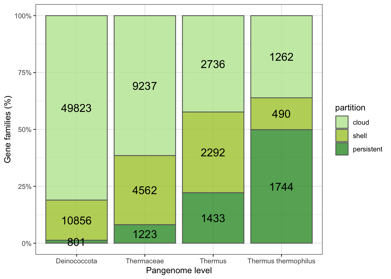
The number of clusters or gene families conserved (Shell+Persistent) increases as we go down in the taxonomical level. Note that the Shell partition shrinks at the species level, suggesting that the identity threshold is probably low at this level for a detailed pangenome analysis. However, as we will focus in the Persistent partition, the calculated pangenomes would be enough informative.
As mentioned above, in order to compute the pangenomes, we carried out a new annotation of the genes in all the assemblies. This is required to have homogeneous gene definitions, but that also gives rise to some differences between the classical NCBI Genbank annotation that we used for the pangenome and the new annotations. Thus, in order to integrate the HB27 genes from TnSeq (TT_CXXXX) and pangenome genes (GCF_000008125.1_XXXXX) in the same table, we used the package fuzzyjoin that allows a flexible merge of the data, considering the gene start and stop as an interval rather than fixed coordinates. However, this flexibility also has a price, as we have some pangenome genes that matched with more than one gene in the classical annotation. We tested different levels of flexibility in the coordinates to maximize the number of genes in the table and at the same time minimize the number of duplicates.
#cross GCA_000008125.1 in all pangenomes
matrix <- list()
HB27 <- data.frame()
for (i in 1:length(pangenomes)){
  matrix[[i]]<- read.table(paste0("pangenomes/",pangenomes[i],"/table/GCF_000008125.1.tsv"),header=TRUE,sep="\t")
}
HB27 <- merge(matrix[[1]][,c(1:4,8)],matrix[[2]][,c(1:4,8)],by=c("gene","contig","start","stop"),all=TRUE)
colnames(HB27)[5:6] <- pangenomes[1:2]
HB27 <- merge(HB27,matrix[[3]][,c(1:4,8)],by=c("gene","contig","start","stop"),all=TRUE)
HB27 <- merge(HB27,matrix[[4]][,c(1:4,8)],by=c("gene","contig","start","stop"),all=TRUE)
colnames(HB27)[7:8] <- pangenomes[3:4]

#cross gene names
tnseq <- read.csv2("tnSeq_dd_full.csv")
HB27_genome <- read.table("00_raw/refs/GCA_000008125.1.gtf",sep="\t",header=FALSE)
HB27_genome$Chr <- "AE017221.1"
HB27_genome$Chr[8088:nrow(HB27_genome)] <- "AE017222.1"
HB27_genome$V9 <-  substr(HB27_genome$V9,9,16)
colnames(HB27_genome)[c(4:5,9)] <- c("start","stop","Genes")
#to reduce differnces in gene annotation, we use fuzzyjoin
#we use the highest max_dist value that don't give rise to duplicate gene names
tmp <- fuzzyjoin::difference_inner_join(HB27[HB27$contig=="contig_1",],HB27_genome[HB27_genome$V3=="CDS" & HB27_genome$V1=="AE017221.1" ,c(4:5,9)], by =c("start", "stop"), max_dist = 210 )
tmp2 <- fuzzyjoin::difference_inner_join(HB27[HB27$contig=="contig_2",],HB27_genome[HB27_genome$V3=="CDS" & HB27_genome$V1=="AE017222.1" ,c(4:5,9)], by =c("start", "stop"), max_dist = 210 )
HB27_annotated <- rbind(tmp,tmp2)

#now we fetch the number of genomes with members in each family and paralogs
#load pangenome matrix
matrix <- list()
for (i in 1:length(pangenomes)){
  matrix[[i]]<- read.table(paste0("pangenomes/",pangenomes[i],"/matrix.csv"),sep=",",header=TRUE)
  matrix[[i]] <- matrix[[i]][,c(4,6,match("GCF_000008125.1",names(matrix[[i]])))]
  colnames(matrix[[i]])[3] <- "gene"

  #for (j in 1:nrow(HB27_annotated)){
  #  k <- grep(HB27_annotated$gene[j],matrix[[i]]$gene)
  #  HB27_annotated$isolates[j] <- matrix[[i]]$No..isolates[k]
  #  HB27_annotated$seqs[j] <- matrix[[i]]$Avg.sequences.per.isolate[k]
  #}
  HB27_annotated$isolates <- sapply(1:nrow(HB27_annotated), function(j) {
  k <- grep(HB27_annotated$gene[j], matrix[[i]]$gene)
  matrix[[i]]$No..isolates[k]
  })
  HB27_annotated$seqs <- sapply(1:nrow(HB27_annotated), function(j) {
  k <- grep(HB27_annotated$gene[j], matrix[[i]]$gene)
  matrix[[i]]$Avg.sequences.per.isolate[k]
  })
  colnames(HB27_annotated)[c(length(HB27_annotated)-1,length(HB27_annotated))] <- c(paste0(pangenomes[i],"_isolates"),paste0(pangenomes[i],"_seqs.per.isolate"))
}

#final-final table
panTnseq <- merge(tnseq,HB27_annotated[,c(11,5:8,12:19)])
panTnseq_Full <-  merge(tnseq,HB27_annotated[,c(11,5:8,12:19)],by="Genes",all.x=TRUE)
#reorder columns and save
setcolorder(panTnseq_Full,"cluster",before ="Ppol_1")
#combine description fields
panTnseq_Full$Description.y[panTnseq_Full$Description.y=="-"] <- panTnseq_Full$Description.x[panTnseq_Full$Description.y=="-"]
setcolorder(panTnseq_Full,"Description.y",before ="Description.x")
panTnseq_Full <- panTnseq_Full[,-5]
names(panTnseq_Full)[4] <- "Description"
#save
#fwrite(panTnseq_Full,"tnseq_pangenome_25feb2025.csv",sep=";", row.names = FALSE)
#writexl::write_xlsx(panTnseq_Full,"tnseq_pangenome_25feb2025.xlsx")
We have been able to match in the pangenome 2190 genes out of 2275, with only 3 genes of the newly annotated HB27 (GCF_000008125.1_07995, GCF_000008125.1_08920, and GCF_000008125.1_08925) that matched with two genes in the classical annotation (TT_CXXXX).
The final table is saved as tnseq_pangenome_25feb2025.xlsx
There’s no overall correlation between the TnSeq group classification of the HB27 genes, with the number of conserved genes in each pangenome and the pangenome cluster.
#recuento

high <- c()
intermediate <- c()
less <- c()
for (i in 1:4){
  high[i] <- nrow(subset(panTnseq,panTnseq[,17+i]=="persistent"  & panTnseq$cluster=="Highly Permissive" ))
   intermediate[i] <- nrow(subset(panTnseq,panTnseq[,17+i]=="persistent" & panTnseq$cluster=="Intermediate" ))
   less[i] <- nrow(subset(panTnseq,panTnseq[,17+i]=="persistent" & panTnseq$cluster=="Less Permissive" ))
}
stats <- data.frame(high,intermediate,less)
row.names(stats) <- names(pangenomes)
stats <- cbind(row.names(stats),stack(stats))
names(stats) <- c("level","ratio","cluster")
#plot
ggplot(stats,aes(x=level, y=ratio,group=cluster)) +
geom_bar(aes(fill=cluster),stat = "identity",position="fill",color="grey40", alpha=0.8) + ylab("Pangenome Persistent Genes (%)")+ geom_text(aes(label=ratio),size=5, position = position_fill(vjust=0.5) , col = "black")+xlab("Pangenome level") +scale_y_continuous(labels = scales::percent) +theme_bw()+ theme(axis.text.x = element_text(angle = 45,vjust=1,hjust=1),text=element_text(face="bold"))+labs(fill="TnSeq gene group")+scale_fill_manual(labels=c("Highly permissive","Intermediate","Less Permissive"),values=c("#FF9966", "#619CFF" ,"#3366CC")) 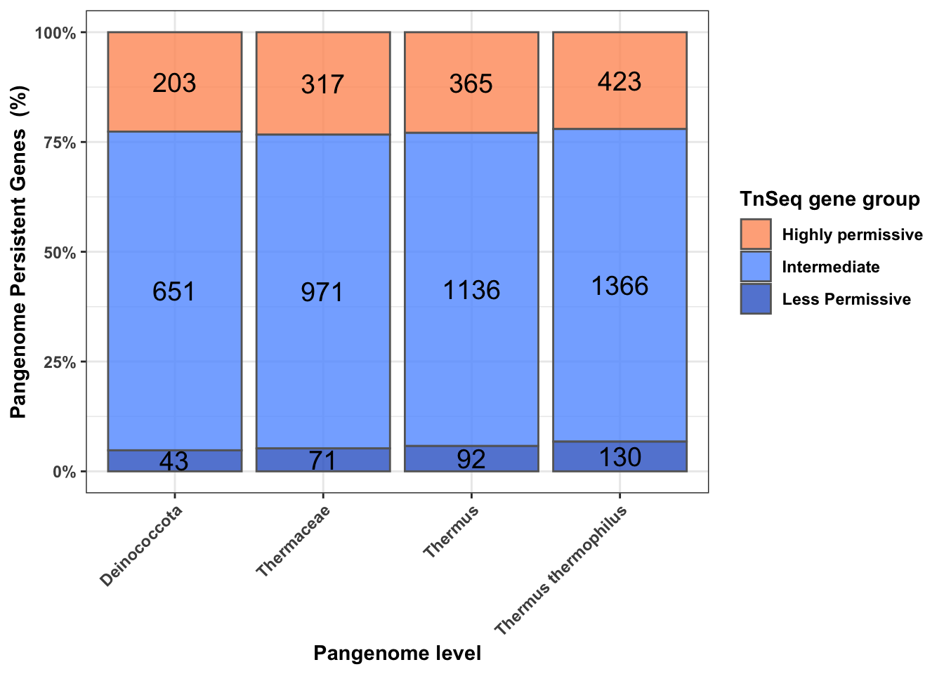
ggsave("fig4b.pdf",width=5,height=5)Now, let’s see genes distribution in the different groups using Venn diagrams.
       x <- list(
  Intermediate = panTnseq_Full$Genes[panTnseq_Full$cluster=="Intermediate"],
  Highly_permissive = panTnseq_Full$Genes[panTnseq_Full$cluster=="Highly Permissive"],
  Less_permissive = panTnseq_Full$Genes[panTnseq_Full$cluster=="Less Permissive"],
  Persistent = panTnseq_Full$Genes[panTnseq_Full$tt_i4c5=="persistent"]
  )

library(ggvenn)
Loading required package: gridtt <- ggvenn(
x,
fill_color = c("#EFC000FF","#0073C2FF","cornflowerblue", "#CD534CFF"),
stroke_size = 0.5, set_name_size = 4
) + ggtitle("Thermus thermophilus") + theme(plot.title = element_text(hjust = 0.5))+
scale_x_continuous(expand = expansion(mult = c(0.15, 0.15)))
x[[4]] <- panTnseq_Full$Genes[panTnseq_Full$thermus_i4c5=="persistent"]
thermus <- ggvenn(
x,
fill_color = c("#EFC000FF","#0073C2FF","cornflowerblue", "#CD534CFF"),
stroke_size = 0.5, set_name_size = 4
) + ggtitle("Thermus") + theme(plot.title = element_text(hjust = 0.5))+
scale_x_continuous(expand = expansion(mult = c(0.15, 0.15)))
x[[4]] <- panTnseq_Full$Genes[panTnseq_Full$thermaceae_i4c5=="persistent"]
thermaceae <- ggvenn(
x,
fill_color = c("#EFC000FF","#0073C2FF","cornflowerblue", "#CD534CFF"),
stroke_size = 0.5, set_name_size = 4
) + ggtitle("Thermaceae") + theme(plot.title = element_text(hjust = 0.5))+
scale_x_continuous(expand = expansion(mult = c(0.15, 0.15)))
x[[4]] <- panTnseq_Full$Genes[panTnseq_Full$deinococcota_i4c5=="persistent"]
deinococcota <- ggvenn(
x,
fill_color = c("#EFC000FF","#0073C2FF","cornflowerblue", "#CD534CFF"),
stroke_size = 0.5, set_name_size = 4
) + ggtitle("Deinococcota") + theme(plot.title = element_text(hjust = 0.5))+
scale_x_continuous(expand = expansion(mult = c(0.15, 0.15)))
ggarrange(tt, thermus, thermaceae, deinococcota,
labels = c("A", "B","C","D"), ncol=2,nrow = 2)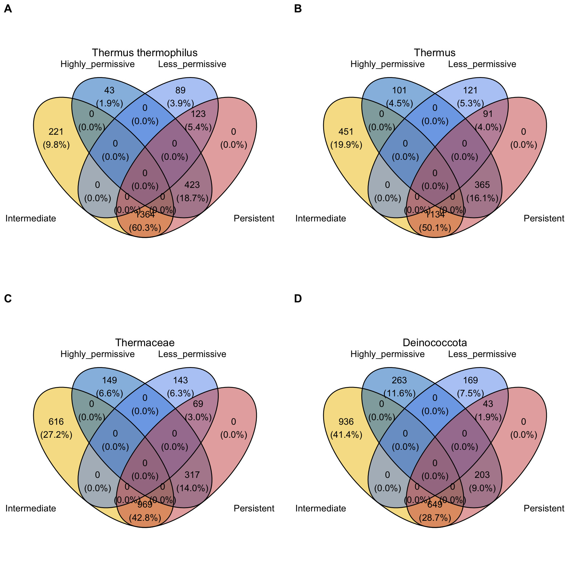
#names(panTnseq_Full)Upset Diagrams allow more detailed comparisons:
colorscale <- c("white","aquamarine","aquamarine1","aquamarine2","aquamarine3","aquamarine4")
colorines <- c("cloud"="#bbe59f","shell"="#abc837","persistent"="#339933","Highly permissive"="#FF9966","Intermediate"="#619CFF" ,"Less permissive"= "#3366CC")
panTnseq_Full[17:20] <- lapply(panTnseq_Full[17:20],factor, levels=c("cloud","shell","persistent"))
library(ggVennDiagram)
Attaching package: 'ggVennDiagram'The following object is masked from 'package:tidyr':
unite#t thermophilus
Tnlist <- append(unstack(panTnseq_Full[,c(1,17)]),unstack(panTnseq_Full[,c(1,10)]))
v1 <- ggVennDiagram(Tnlist,set_color=colorines,label="count",label_alpha=0,show_intersect = FALSE) +
scale_fill_gradientn(colours=colorscale)
u1 <- ggVennDiagram(Tnlist,force_upset = TRUE,order.set.by = "none", order.intersect.by = "none")
#thermus
Tnlist <- append(unstack(panTnseq_Full[,c(1,18)]),unstack(panTnseq_Full[,c(1,10)]))
v2 <- ggVennDiagram(Tnlist,set_color=colorines,label="count",label_alpha=0,show_intersect = FALSE)+
scale_fill_gradientn(colours=colorscale)
u2 <- ggVennDiagram(Tnlist,force_upset = TRUE,order.set.by = "none", order.intersect.by = "none")
#thermaceae
Tnlist <- append(unstack(panTnseq_Full[,c(1,19)]),unstack(panTnseq_Full[,c(1,10)]))
v3 <- ggVennDiagram(Tnlist,set_color=colorines,label="count",label_alpha=0,show_intersect = FALSE)+
scale_fill_gradientn(colours=colorscale)
u3 <- ggVennDiagram(Tnlist,force_upset = TRUE,order.set.by = "none", order.intersect.by = "none")
#deino
Tnlist <- append(unstack(panTnseq_Full[,c(1,20)]),unstack(panTnseq_Full[,c(1,10)]))
v4 <- ggVennDiagram(Tnlist,set_color=colorines,label="count",label_alpha=0,show_intersect = FALSE)+
scale_fill_gradientn(colours=colorscale)
u4 <- ggVennDiagram(Tnlist,force_upset = TRUE,order.set.by = "none", order.intersect.by = "none")
#ggarrange(u1+labs(title=expression(italic("T. thermophilus"))), v2+labs(title=expression(italic("Thermus"))), v3+labs(title=expression(italic("Thermaceae"))), v4+labs(title=expression(italic("Deinococcaceae"))), ncol=2,nrow=2,common.legend=TRUE,legend = "bottom")
paste("T. thermophilus")[1] "T. thermophilus"u1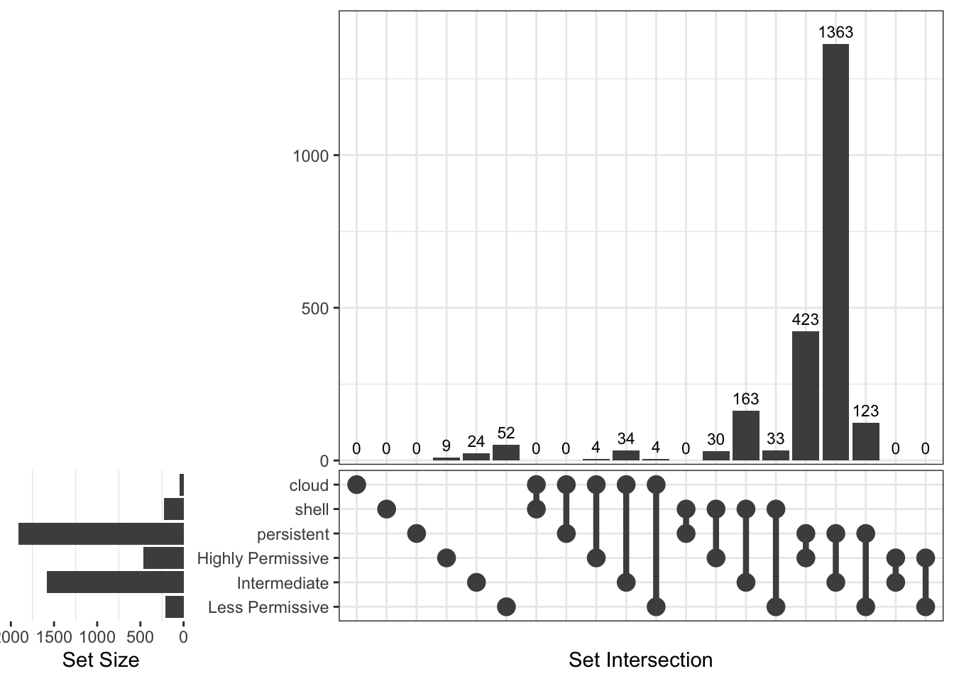
ggsave("Tth_upset.svg",width=4,height=4)
paste("Thermus")
[1] "Thermus"u2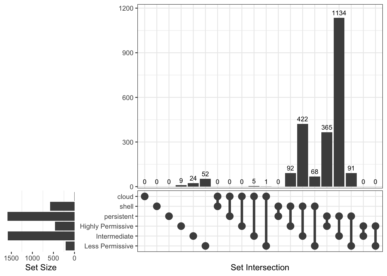
paste("Thermaceae")[1] "Thermaceae"u3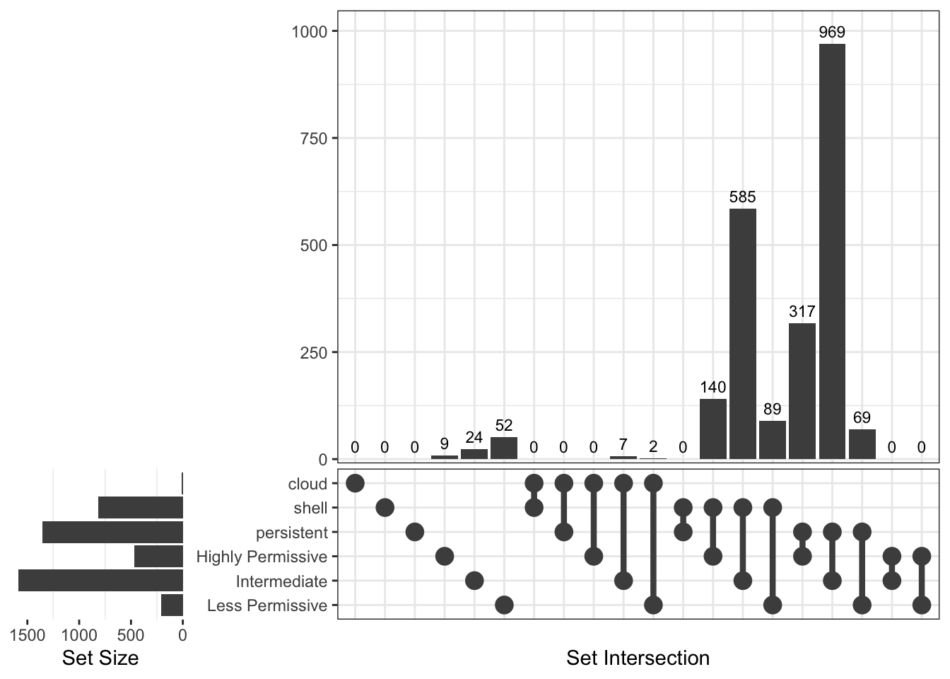
paste("Deinococcota")[1] "Deinococcota"u4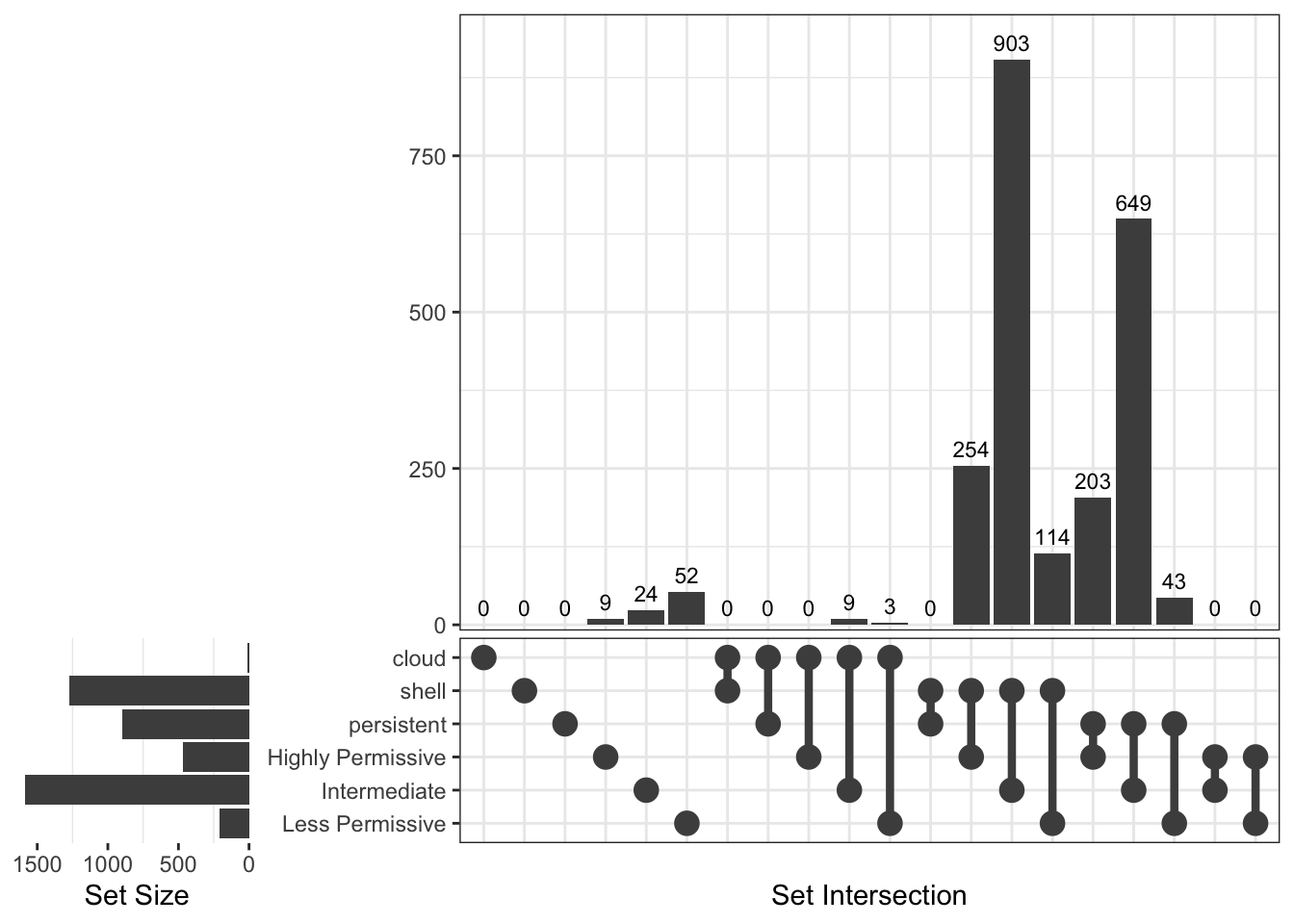
#svg("figure4c.svg")
par(mfrow = c(2, 2),mar=c(1,1,1,1))

#thermus termophilus
Tnmat <- rbind(as.data.frame(as.list(panTnseq_Full[,c(1,10)]),col.names=c("Genes","group")),
               as.data.frame(as.list(panTnseq_Full[,c(1,17)]),col.names=c("Genes","group")))
plot(venneuler(na.omit(Tnmat)),col=c("#FF9966","#619CFF" , "#3366CC","#bbe59f","#abc837","#339933"),alpha=0.7,main=expression(italic("T. thermophilus")))

#thermus
Tnmat <- rbind(as.data.frame(as.list(panTnseq_Full[,c(1,10)]),col.names=c("Genes","group")),
               as.data.frame(as.list(panTnseq_Full[,c(1,18)]),col.names=c("Genes","group")))
plot(venneuler(na.omit(Tnmat)),col=c("#FF9966","#619CFF" , "#3366CC","#bbe59f","#abc837","#339933"),alpha=0.7,main=expression(italic("Thermus")))

#termaceae
Tnmat <- rbind(as.data.frame(as.list(panTnseq_Full[,c(1,10)]),col.names=c("Genes","group")),
               as.data.frame(as.list(panTnseq_Full[,c(1,19)]),col.names=c("Genes","group")))
plot(venneuler(na.omit(Tnmat)),col=c("#FF9966","#619CFF" , "#3366CC","#bbe59f","#abc837","#339933"),alpha=0.7,main=expression(italic("Thermaceae")))

#deinococcota
Tnmat <- rbind(as.data.frame(as.list(panTnseq_Full[,c(1,10)]),col.names=c("Genes","group")),
               as.data.frame(as.list(panTnseq_Full[,c(1,20)]),col.names=c("Genes","group")))
plot(venneuler(na.omit(Tnmat)),col=c("#FF9966","#619CFF" , "#3366CC","#bbe59f","#abc837","#339933"),alpha=0.7,main=expression(italic("Deinococcota")))


dev.off()kk <- enrichKEGG(gene = na.omit(panTnseq_Full[panTnseq_Full$cluster!="Highly Permissive" & panTnseq_Full$thermaceae_i4c5=="persistent",1]),
organism = 'tth',
pvalueCutoff = 0.05)Reading KEGG annotation online: "https://rest.kegg.jp/link/tth/pathway"...Reading KEGG annotation online: "https://rest.kegg.jp/list/pathway/tth"...p1 <- dotplot(kk, title="Thermaceae core genome")
kk_D <- enrichKEGG(gene = na.omit(panTnseq_Full[panTnseq_Full$cluster!="Highly Permissive" & panTnseq_Full$deinococcota_i4c5=="persistent",1]),
organism = 'tth',
pvalueCutoff = 0.05)
p2 <- dotplot(kk_D, title="Deinococcota core genome")
ggarrange(p1, p2,
labels = c("A", "B"), ncol=1,nrow = 2, heights=c(1,1))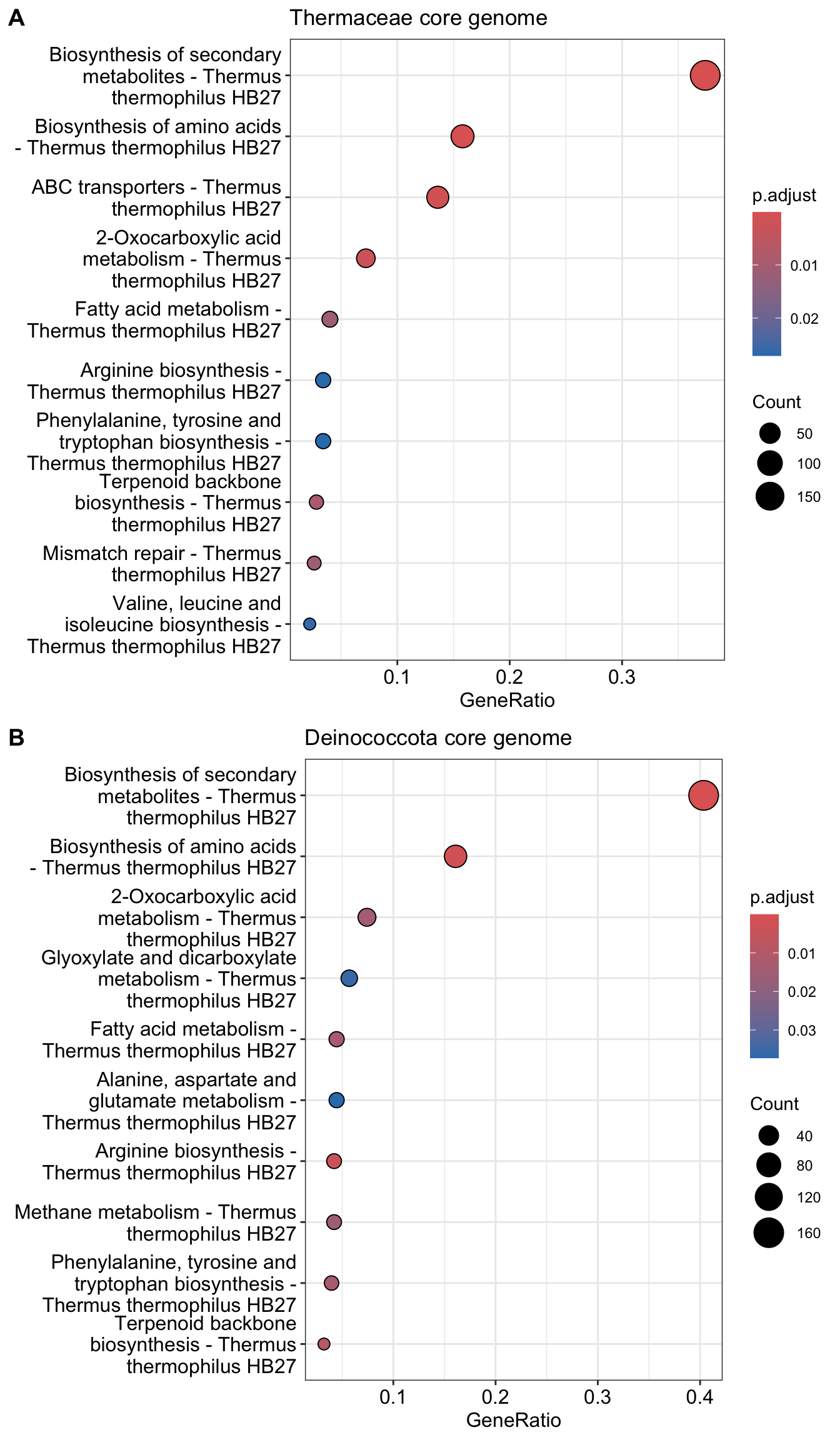
uniprot <- bitr_kegg(panTnseq_Full$Genes, fromType="kegg", toType='uniprot', organism='tth')
panTnseq_Full <- panTnseq_Full %>%
  mutate(uni = replace(Genes, Genes %in% uniprot$kegg, uniprot$uniprot))

kk <- enrichKEGG(gene         = na.omit(panTnseq_Full[panTnseq_Full$cluster!="Highly Permissive"  & panTnseq_Full$thermus_i4c5=="persistent",30]),
           organism     = 'tth', keyType = 'uniprot',
           pvalueCutoff = 0.05)
if (is.null(kk)){
  p1 <- NULL
} else {
  if (any(kk@result$p.adjust<0.05)){
  p1 <- dotplot(kk, title="Thermus core genome")
  } else {
    p1 <- NULL
  }
}

kk_t <- enrichKEGG(gene         = na.omit(panTnseq_Full[panTnseq_Full$cluster!="Highly Permissive"  & panTnseq_Full$thermaceae_i4c5=="persistent",30]),
           organism     = 'tth', keyType = 'uniprot',
           pvalueCutoff = 0.05)
if (is.null(kk_t)){
  p2 <- NULL
} else {
  if (any(kk@result$p.adjust<0.05)){
  p2 <- dotplot(kk_t, title="Thermaceae core genome")
  } else {
    p2 <- NULL
  }
}

kk_D <- enrichKEGG(gene         = na.omit(panTnseq_Full[panTnseq_Full$cluster!="Highly Permissive"  & panTnseq_Full$deinococcota_i4c5=="persistent",30]),
           organism     = 'tth', keyType = 'uniprot',
           pvalueCutoff = 0.05)
if (is.null(kk_D)){
  p3 <- NULL
} else {
  if (any(kk@result$p.adjust<0.05)){
  p3 <- dotplot(kk_D, title="Deinococcota core genome")
  } else {
    p3 <- NULL
  }
}

ggarrange(p1, p2, p3,
labels = c("A", "B", "C"), ncol=1,nrow = 3,heights=c(2,3,3))Since there is no clear correlation between gene conservation and the permissivity of Tn5 insertions, we decided to compare our results with previously published results. We used the data from Zhang et al. (2018) (SUPPLEMENTARY DATA 4), which includes the essential/non-essential genes of a wide range of prokaryotic organisms comprising extremophilic archaea (Sulfolobus islandicus and Methanococcus maripaludis) and various mesophilic bacteria (Bacillus subtilis, Bacteroides fragilis, Escherichia coli) as well as the minimal essential genome of Micoplasma JVCI Syn3.0.
#data from https://www.nature.com/articles/s41467-018-07379-4
essentiality <- read_xlsx("bacteria_essential_genes/41467_2018_7379_MOESM6_ESM.xlsx",sheet=1)
colnames(essentiality)[2] <- "eggNOG_OGs"
panTnseq_Full$eggNOG_OGs <- sub("\\@.*", "", panTnseq_Full$eggNOG_OGs)
world_essential <- merge(panTnseq_Full,essentiality)
#names(world_essential)
 prok <- subset(world_essential,world_essential$`Sulfolobus islandicus M.16.4`=="essential" & world_essential$`Methanococcus maripaludis S2`=="essential" & world_essential$`Bacillus subtilis`=="essential" & world_essential$`Bacteroides fragilis`=="essential" & world_essential$`Escherichia coli`=="essential" & world_essential$`Mycoplasma JCVI Syn3.0`=="essential")
The following table contains the essential genes in all prokaryotic genomes and their HB27 orthologs as annotated by eggNOG. As you can see, out of 53 genes annotated as essentia in all thouse prokaryotic organisms, 6 were Highly Permissive and 27 (50.9%) Intermediate in HB27 TnSeq, but they are again highly conserved as all of them are persistent genes in the T. thermophilus pangenome and near 92.5% are still members of the core genome of Deinococcota pangenome.
datatable(prok[,c(1,2,10,17:20)],rownames = FALSE, escape = FALSE, filter="top", extensions = 'Responsive',options = list( pageLength = 25, autoWidth = TRUE ))#table to save
library(kableExtra)
Attaching package: 'kableExtra'The following object is masked from 'package:dplyr':
group_rowskbl(prok[,c(1,4,10,17:20)], align = "c", row.names = FALSE,col.names= c("eggNOG","Description","TnSeq","T. thermophilus","Thermus","Thermaceae","Deinococcota"), caption = "Table 2. Tth TnSeq and Pangenome analysis of selected prokaryotic essential genes from diverse previous works (Zhang et al. 2018). See Methods for details.", "html") %>%
kable_styling(bootstrap_options = "condensed", full_width = F, position = "center") %>%
column_spec(1, bold = T, italic=F) #%>% save_kable("table2_new.pdf",self_contained=TRUE)| eggNOG | Description | TnSeq | T. thermophilus | Thermus | Thermaceae | Deinococcota |
|---|---|---|---|---|---|---|
| COG0008 | Glutamate--tRNA ligase | Intermediate | persistent | persistent | persistent | persistent |
| COG0008 | Glutamine--tRNA ligase | Intermediate | persistent | persistent | persistent | persistent |
| COG0013 | Alanine--tRNA ligase | Intermediate | persistent | shell | shell | shell |
| COG0016 | Phenylalanine--tRNA ligase alpha subunit | Highly Permissive | persistent | persistent | persistent | persistent |
| COG0017 | Aspartate--tRNA(Asp/Asn) ligase | Intermediate | persistent | persistent | persistent | persistent |
| COG0017 | Asparagine--tRNA ligase | Less Permissive | persistent | persistent | persistent | persistent |
| COG0018 | Arginine--tRNA ligase | Intermediate | persistent | persistent | persistent | persistent |
| COG0024 | Methionine aminopeptidase | Less Permissive | persistent | persistent | persistent | shell |
| COG0048 | 30S ribosomal protein S12 | Less Permissive | persistent | persistent | persistent | persistent |
| COG0049 | 30S ribosomal protein S7 | Less Permissive | persistent | persistent | persistent | persistent |
| COG0051 | 30S ribosomal protein S10 | Less Permissive | persistent | persistent | persistent | persistent |
| COG0052 | 30S ribosomal protein S2 | Intermediate | persistent | persistent | persistent | persistent |
| COG0060 | Isoleucine--tRNA ligase | Intermediate | persistent | persistent | persistent | persistent |
| COG0081 | 50S ribosomal protein L1 | Intermediate | persistent | persistent | persistent | persistent |
| COG0087 | 50S ribosomal protein L3 | Intermediate | persistent | persistent | persistent | persistent |
| COG0088 | 50S ribosomal protein L4 | Less Permissive | persistent | persistent | persistent | persistent |
| COG0089 | 50S ribosomal protein L23 | Intermediate | persistent | persistent | persistent | persistent |
| COG0090 | 50S ribosomal protein L2 | Less Permissive | persistent | persistent | persistent | persistent |
| COG0091 | 50S ribosomal protein L22 | Less Permissive | persistent | persistent | persistent | persistent |
| COG0094 | 50S ribosomal protein L5 | Less Permissive | persistent | persistent | persistent | persistent |
| COG0096 | 30S ribosomal protein S8 | Less Permissive | persistent | persistent | persistent | persistent |
| COG0097 | 50S ribosomal protein L6 | Intermediate | persistent | persistent | persistent | persistent |
| COG0098 | 30S ribosomal protein S5 | Less Permissive | persistent | persistent | persistent | persistent |
| COG0099 | 30S ribosomal protein S13 | Less Permissive | persistent | persistent | persistent | persistent |
| COG0100 | 30S ribosomal protein S11 | Less Permissive | persistent | persistent | persistent | persistent |
| COG0102 | 50S ribosomal protein L13 | Intermediate | persistent | persistent | persistent | persistent |
| COG0103 | 30S ribosomal protein S9 | Less Permissive | persistent | persistent | persistent | persistent |
| COG0124 | Histidine--tRNA ligase | Less Permissive | persistent | shell | persistent | persistent |
| COG0162 | Tyrosine--tRNA ligase | Highly Permissive | persistent | persistent | persistent | persistent |
| COG0172 | Serine--tRNA ligase | Less Permissive | persistent | persistent | persistent | persistent |
| COG0180 | Tryptophan--tRNA ligase | Intermediate | persistent | persistent | persistent | persistent |
| COG0186 | 30S ribosomal protein S17 | Less Permissive | persistent | persistent | persistent | persistent |
| COG0195 | Transcription termination/antitermination protein NusA | Intermediate | persistent | persistent | persistent | persistent |
| COG0197 | 50S ribosomal protein L16 | Less Permissive | persistent | persistent | persistent | persistent |
| COG0198 | 50S ribosomal protein L24 | Intermediate | persistent | persistent | persistent | persistent |
| COG0199 | 30S ribosomal protein S14 type Z | Less Permissive | persistent | persistent | persistent | persistent |
| COG0201 | Protein translocase subunit SecY | Intermediate | persistent | persistent | persistent | persistent |
| COG0202 | DNA-directed RNA polymerase subunit alpha | Intermediate | persistent | persistent | persistent | persistent |
| COG0256 | 50S ribosomal protein L18 | Intermediate | persistent | persistent | persistent | persistent |
| COG0361 | Translation initiation factor IF-1 | Intermediate | persistent | persistent | persistent | persistent |
| COG0442 | Proline--tRNA ligase | Highly Permissive | persistent | persistent | persistent | persistent |
| COG0462 | Ribose-phosphate pyrophosphokinase | Highly Permissive | persistent | persistent | persistent | persistent |
| COG0462 | Ribose-phosphate pyrophosphokinase | Intermediate | persistent | persistent | persistent | persistent |
| COG0470 | DNA polymerase III subunit delta' | Intermediate | persistent | persistent | persistent | shell |
| COG0470 | DNA polymerase III | Intermediate | persistent | shell | shell | shell |
| COG0480 | Elongation factor G | Highly Permissive | persistent | persistent | persistent | persistent |
| COG0480 | Elongation factor G | Intermediate | persistent | persistent | persistent | persistent |
| COG0495 | Leucine--tRNA ligase | Highly Permissive | persistent | persistent | persistent | persistent |
| COG0504 | CTP synthase | Intermediate | persistent | persistent | persistent | persistent |
| COG0522 | 30S ribosomal protein S4 | Less Permissive | persistent | persistent | persistent | persistent |
| COG0525 | Valine--tRNA ligase | Intermediate | persistent | persistent | persistent | persistent |
| COG0532 | Translation initiation factor IF-2 | Intermediate | persistent | persistent | persistent | persistent |
| COG0592 | Beta sliding clamp | Intermediate | persistent | persistent | persistent | persistent |
To quantify the correlation between Tn-seq, gene conservation in pangenomes and gene essentiality, we used the data from Rancati et al. (2018), which compares the gene essentiality in diverse bacteria from diverse works. Thus, we downloaded the data from the papers indicated below and parsed the essential genes. To unify nomenclature, we tried to obtain the EggNOG COG code for each gene and used it to merge genes with different names across the different species. All data was parsed with an external R script to generate a common table (all_essentials.csv).
| Strain | Ref. PMID | Assembly | FileName |
|---|---|---|---|
| E. coli K12 | 29463657 | GCF_000800765.1 | mbo001183726st1.xlsx |
| M. tuberculosis H37Rv | 28096490 | GCF_000195955.2 | mbo002173137st3.xlsx |
| M. genitalum G37 | 16407165 | GCA_000027325.1 | pnas_0510013103_10013Table2.xls |
| P. aerugionsa PAO1 | 25848053 | GCF_000006765.1 | pnas.1422186112.sd01.xlsx |
| S. aureus HG003 | 25888466 | GCF_000013425.1 | 12864_2015_1361_MOESM2_ESM.xlsx |
| S. pyogenes (5448 & NZ131) | 25996237 | GCA_000011765.2 | srep09838-s1.pdf (Table S3!) |
| Synechococcus elongatus PCC 7942 | 26508635 | GCF_000012525.1 | pnas.1519220112.sd03.xlsx |
First, we evaluate the correlation between the essential/indispensable genes with our HB27 TnSeq and pangenome data. As shown below, despite the fact that the bacterial data come from different sources, we see some negative correlation between the number of genomes with essential and dispensable genes. In addition, there is also a moderate positive correlation between gene essentiality and conservation in our pangenome. However, consistent with previous results, the TnSeq results do not correlate with other analyses, suggesting that T. thermophilus is reluctant to reveal its essential genes.
Finally, we compared Tn-seq, pangenome and transcriptome of HB27 with the abovementioned prokaryotic “essentialtome”. We used the data from Swarts et al. (2015) that contains triplicate data of gene expression in HB27. The expression level was also used for correlation analysis.
#data from https://www.nature.com/articles/s41467-018-07379-4

essential_mix <- read.csv2("bacteria_essential_genes/all_essentials.csv")
world_essential <- merge(world_essential,essential_mix,by="eggNOG_OGs")
fwrite(world_essential,"bacteria_essential_genes/all_essentials_panTnseq_25feb25.csv", sep=";")


#add rnaseq in HB27
rnaseq <- read_xlsx("bacteria_essential_genes/pone.0124880.s002.xlsx",sheet=1)
names(rnaseq)[2] <- "Genes"
panTnseq_Full2 <-  merge(world_essential,rnaseq[,c(2,7:9)],by="Genes",all.x=TRUE)
panTnseq_Full2[,c(11:16,21:28,50:54)] <- lapply(panTnseq_Full2[,c(11:16,21:28,50:54)], as.numeric)

M <-cor(panTnseq_Full2[,c(11:14,22,24,26,28,50:54)], method = "spearman", use = "pairwise.complete.obs")
testRes <-  cor.mtest(panTnseq_Full2[,c(11:14,22,24,26,28,50:54)], conf.level = 0.99)
corrplot(M, type="lower", p.mat = testRes$p, method = 'circle', insig='blank',
         tl.col="black",tl.srt = 45, addCoef.col ='black', number.cex = 0.5,tl.cex=0.5, col=brewer.pal(n=8, name="Spectral"))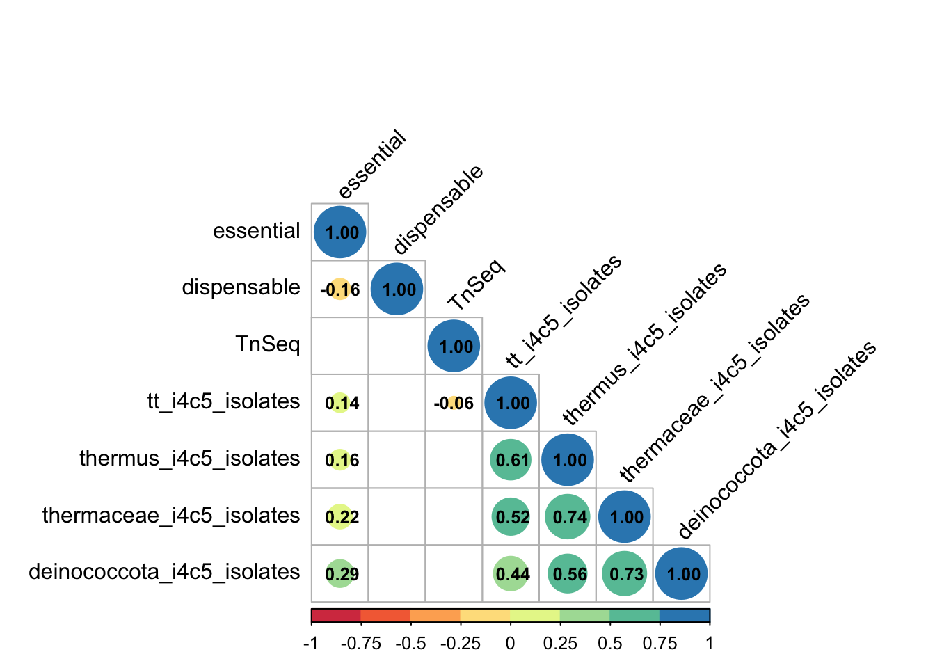
The detailed table of bacteria essential genes and HB27 TnSeq+Pangenome data can be found in file all_essentials_panTnseq.csv.
ggplot(as.data.frame(table(world_essential$essential,world_essential$cluster)),aes(x=Var1, y=Freq,group=Var2)) +
         geom_bar(aes(fill=Var2),stat = "identity",position="fill",color="grey40", alpha=0.8) +  geom_text(aes(label=Freq),size=4, position = position_fill(vjust=0.5) , col = "black")+ xlab("Number genomes with each essential gene") + ylab("TnSeq group (%)") +scale_y_continuous(labels = scales::percent) + theme_bw()+ labs(fill = "TnSeq group")
Overall, multiple correlation analysis shows a moderate correlation between expression levels and ortholog gene essentiality, but slight negative correlation with Tn-seq Z-score. Thus, highly transcribed genes in HB27 are abundant within the highly conserved (persistent) group and overall they would get somewhat less hits in our Tn-seq. Altogether, these results indicate that despite the different lifestyles and phylogenetic distances among the genomes examined in prior essentiality studies, the expected higher conservation of universally essential genes is applicable to Tth, even though, in this case, the Tn-seq approach may not readily disclose most of essential genes.
sessionInfo()R version 4.4.1 (2024-06-14)
Platform: x86_64-apple-darwin20
Running under: macOS Sonoma 14.6.1
Matrix products: default
BLAS: /Library/Frameworks/R.framework/Versions/4.4-x86_64/Resources/lib/libRblas.0.dylib
LAPACK: /Library/Frameworks/R.framework/Versions/4.4-x86_64/Resources/lib/libRlapack.dylib; LAPACK version 3.12.0
locale:
[1] en_US.UTF-8/en_US.UTF-8/en_US.UTF-8/C/en_US.UTF-8/en_US.UTF-8
time zone: Europe/Madrid
tzcode source: internal
attached base packages:
[1] grid stats graphics grDevices utils datasets methods
[8] base
other attached packages:
[1] kableExtra_1.4.0 ggVennDiagram_1.5.2 ggvenn_0.1.10
[4] venneuler_1.1-4 rJava_1.0-11 readxl_1.4.3
[7] ggpubr_0.6.0 clusterProfiler_4.13.4 RColorBrewer_1.1-3
[10] corrplot_0.95 ggstats_0.7.0 patchwork_1.3.0
[13] lubridate_1.9.3 forcats_1.0.0 stringr_1.5.1
[16] purrr_1.0.2 readr_2.1.5 tidyr_1.3.1
[19] tibble_3.2.1 tidyverse_2.0.0 dplyr_1.1.4
[22] DT_0.33 data.table_1.16.2 ggplot2_3.5.1
[25] formatR_1.14 knitr_1.48
loaded via a namespace (and not attached):
[1] rstudioapi_0.17.1 jsonlite_1.8.9 magrittr_2.0.3
[4] ggtangle_0.0.3 farver_2.1.2 rmarkdown_2.28
[7] ragg_1.3.3 fs_1.6.5 zlibbioc_1.51.2
[10] vctrs_0.6.5 memoise_2.0.1 ggtree_3.13.2
[13] rstatix_0.7.2 htmltools_0.5.8.1 broom_1.0.7
[16] cellranger_1.1.0 Formula_1.2-5 gridGraphics_0.5-1
[19] sass_0.4.9 bslib_0.8.0 htmlwidgets_1.6.4
[22] plyr_1.8.9 cachem_1.1.0 igraph_2.1.1
[25] lifecycle_1.0.4 pkgconfig_2.0.3 fuzzyjoin_0.1.6
[28] Matrix_1.7-1 R6_2.5.1 fastmap_1.2.0
[31] gson_0.1.0 GenomeInfoDbData_1.2.13 digest_0.6.37
[34] aplot_0.2.3 enrichplot_1.25.5 colorspace_2.1-1
[37] AnnotationDbi_1.67.0 S4Vectors_0.43.2 crosstalk_1.2.1
[40] textshaping_0.4.0 RSQLite_2.3.7 labeling_0.4.3
[43] fansi_1.0.6 timechange_0.3.0 httr_1.4.7
[46] abind_1.4-8 compiler_4.4.1 bit64_4.5.2
[49] withr_3.0.2 backports_1.5.0 BiocParallel_1.39.0
[52] carData_3.0-5 DBI_1.2.3 highr_0.11
[55] R.utils_2.12.3 ggsignif_0.6.4 tools_4.4.1
[58] ape_5.8 R.oo_1.26.0 glue_1.8.0
[61] nlme_3.1-166 GOSemSim_2.31.2 reshape2_1.4.4
[64] fgsea_1.31.6 generics_0.1.3 gtable_0.3.6
[67] tzdb_0.4.0 R.methodsS3_1.8.2 hms_1.1.3
[70] xml2_1.3.6 car_3.1-3 utf8_1.2.4
[73] XVector_0.45.0 BiocGenerics_0.51.3 ggrepel_0.9.6
[76] pillar_1.9.0 yulab.utils_0.1.7 vroom_1.6.5
[79] splines_4.4.1 treeio_1.29.2 lattice_0.22-6
[82] bit_4.5.0 tidyselect_1.2.1 GO.db_3.20.0
[85] Biostrings_2.73.2 IRanges_2.39.2 svglite_2.1.3
[88] stats4_4.4.1 xfun_0.48 Biobase_2.65.1
[91] stringi_1.8.4 UCSC.utils_1.1.0 lazyeval_0.2.2
[94] ggfun_0.1.7 yaml_2.3.10 evaluate_1.0.1
[97] codetools_0.2-20 qvalue_2.37.0 ggplotify_0.1.2
[100] cli_3.6.3 systemfonts_1.1.0 jquerylib_0.1.4
[103] munsell_0.5.1 Rcpp_1.0.13 GenomeInfoDb_1.41.2
[106] png_0.1-8 parallel_4.4.1 blob_1.2.4
[109] DOSE_3.99.1 viridisLite_0.4.2 tidytree_0.4.6
[112] scales_1.3.0 crayon_1.5.3 rlang_1.1.4
[115] cowplot_1.1.3 fastmatch_1.1-4 KEGGREST_1.45.1