Thermus TnSeq
  • Home
  • Contents
    • TnSeq Illumina Data Processing
    • TnSeq Genes classification
    • Thermus Pangenome

On this page

  • Raw data processing
  • Reads Mapping Analysis
    • Mapping stats
    • Mapping coverage in HB27 genome
  • Tn5 transposon insertions per gene and Z-score
    • Count integration events counts per gene and Z-score calculation
    • Summary stats
    • Insertions in key genes

TnSeq Illumina Data Processing

Author
Affiliation

Modesto

Department of Biochemistry, UAM

Published

April 26, 2024

Modified

March 28, 2025

Raw data processing

Quality check, reads filtering, trimming and deduplication was carried out with FastP 0.23.4 Chen et al. (2018) and reports were merged with MultiQC 1.22.3. Reads processing parameters were optimized to maximal proportion of mapped reads against the reference HB27 assembly GCA_0000081251.

Show code
conda activate bioconda
conda install -c bioconda fastp
#fastp 0.23.4

cd data/Tnseq_thermus
mkdir 00_fastp
fastp -i 00_raw/TNB-03_S3_L001_R1_001.fastq.gz -a TAAGAGACAGTCTAGA -o 00_fastp/TNB-03_trimmed_dd.fastq -f 30 -t 10 -g -D -h 00_fastp/TNB_03_dd.html -j 00_fastp/TNB_03_fastp_dd.json -q 20 -r --cut_right_window_size 10 --cut_right_mean_quality 30 -w 10
fastp -i 00_raw/TNB-01_S1_L001_R1_001.fastq.gz -a TAAGAGACAGTCTAGA -o 00_fastp/TNB-01_trimmed_dd.fastq -f 30 -t 10 -g -D -h 00_fastp/TNB_01_dd.html -j 00_fastp/TNB_01_fastp_dd.json -q 20 -r --cut_right_window_size 10 --cut_right_mean_quality 30 -w 10
fastp -i 00_raw/TNB-07_S3_L001_R1_001.fastq.gz -a TAAGAGACAGTCTAGA -o 00_fastp/TNB-07_trimmed_dd.fastq -f 30 -t 10 -g -D -h 00_fastp/TNB_07_dd.html -j 00_fastp/TNB_07_fastp_dd.json -q 20 -r --cut_right_window_size 10 --cut_right_mean_quality 30 -w 10
fastp -i 00_raw/TNB-09_S5_L001_R1_001.fastq.gz -a TAAGAGACAGTCTAGA -o 00_fastp/TNB-09_trimmed_dd.fastq -f 30 -t 10 -g -D -h 00_fastp/TNB_09_dd.html -j 00_fastp/TNB_09_fastp_dd.json -q 20 -r --cut_right_window_size 10 --cut_right_mean_quality 30 -w 10

cd 00_fastp
mkdir reports_dd
mv *.json reports_dd
mv *.html reports_dd

conda activate base
multiqc -v reports_dd

The statistics of the final reads, after QC-filtering and dedupication, are shown in the Table 1 below. The detailed FastP combined reports is available here.

Show code
fastp <- read.table("00_fastp/merged_fastp_reports.csv", header = TRUE, sep = ";")
fastp$Sample <- c("Ppol_1","HB27_1","HB27_2","Ppol_2")
fastp$initial_reads <- c(2170192,3196758,1515716, 1820971)
my.cols <- brewer.pal(4, "Paired")
kbl(fastp[c(1,4,2,3),c(1,2,8,3,4,6,5)], align = "c", row.names = FALSE,col.names= c("Library","File","Reads","% Duplication","Final reads (M)","Final reads (%)","GC %"), caption = "Table 1. Statistics of fastp processed reads of HB27 TnSeq libraries") %>%
    kable_styling(bootstrap_options = "striped", full_width = F, position = "center") %>%
    column_spec(1, bold = T, italic=T, color=my.cols)
Table 1. Statistics of fastp processed reads of HB27 TnSeq libraries
Library File Reads % Duplication Final reads (M) Final reads (%) GC %
Ppol_1 TNB-01_S1_L001_R1_001 2170192 78.20% 0.9 41.40% 59.40%
Ppol_2 TNB-09_S5_L001_R1_001 1820971 78.60% 1.7 92.10% 64.90%
HB27_1 TNB-03_S3_L001_R1_001 3196758 72.40% 2.7 83.90% 65.40%
HB27_2 TNB-07_S3_L001_R1_001 1515716 74.20% 1.3 88.30% 65.80%

The original sample looks slightly different, with less reads and length, as well as somewhat lower GC content. Note that HB27 chromosome has 1.894.877 bp and 69.5% GC and pTT27 has 232.605 and 69% GC.

Given that several samples were sequenced in the same batch, downplaying a technical problem with sequencing library o running, we hypothesize that some transposon insertions may be unstable in the context of Thermus.

Reads Mapping Analysis

Mapping stats

Filtered reads were mapped using Bowtie2 2.5.1.

Show code
cd 00_raw/refs
bowtie2-build GCA_000008125.fa HB27_gb
cd ..

(bowtie2 -x 00_raw/refs/HB27_gb --no-unal --very-sensitive -U 00_fastp/TNB-03_trimmed_dd.fastq -p 10 | samtools view -bS - | samtools sort -@ 12 -o 01_bowtie2/mapping_TNB03_dd_sorted.bam) 2> TNB-03_dd_mapping.log

(bowtie2 -x 00_raw/refs/HB27_gb --no-unal --very-sensitive -U 00_fastp/TNB-07_trimmed_dd.fastq -p 10 | samtools view -bS - | samtools sort -@ 12 -o 01_bowtie2/mapping_TNB07_dd_sorted.bam) 2> TNB-07_dd_mapping.log

(bowtie2 -x 00_raw/refs/HB27_gb --no-unal --very-sensitive -U 00_fastp/TNB-01_trimmed_dd.fastq -p 10 | samtools view -bS - | samtools sort -@ 12 -o 01_bowtie2/mapping_TNB01_dd_sorted.bam) 2> TNB-01_dd_mapping.log

(bowtie2 -x 00_raw/refs/HB27_gb --no-unal --very-sensitive -U 00_fastp/TNB-09_trimmed_dd.fastq -p 10 | samtools view -bS - | samtools sort -@ 12 -o 01_bowtie2/mapping_TNB09_dd_sorted.bam) 2> TNB-09_dd_mapping.log

Let’s have a look to the data from bowtie2 alignment reports and the average stats obtained with Weesam 1.6.

Show code
#read bowtie stats
bowtie2 <- read.table("01_bowtie2/bowtie2_stats.csv",sep=";",header=TRUE)
bowtie2 <- cbind(bowtie2[,c(1,4)],stack(bowtie2[,2:3]))
bowtie2$library <- ifelse(bowtie2$sample=="TNB01","Ppol_1",ifelse(bowtie2$sample=="TNB07","Ppol_2",ifelse(bowtie2$sample=="TNB03","HB27_1","HB27_2")))
bowtie2$library <- factor(bowtie2$library, levels=c("Ppol_1","Ppol_2","HB27_1","HB27_2"))
#read and combine  weesam data
weesam <- read.table("01_bowtie2/weeSAM_reports/TNB01.txt", sep="\t", header=TRUE)
weesam <- rbind(weesam, read.table("01_bowtie2/weeSAM_reports/TNB09.txt", sep="\t",header=TRUE), read.table("01_bowtie2/weeSAM_reports/TNB03.txt", sep="\t",header=TRUE), read.table("01_bowtie2/weeSAM_reports/TNB07.txt", sep="\t",header=TRUE))
weesam$sample <- c("TNB01","TNB01","TNB09","TNB09","TNB03","TNB03","TNB07","TNB07")
weesam$library <- ifelse(weesam$sample=="TNB01","Ppol_1",ifelse(weesam$sample=="TNB07","Ppol_2",ifelse(weesam$sample=="TNB03","HB27_1","HB27_2")))
weesam$library <- factor(weesam$library, levels=c("Ppol_1","Ppol_2","HB27_1","HB27_2"))
weesam$aligned <- c()
#plots
g1 <-ggplot(bowtie2)+geom_bar(aes(x=library,y=values, fill=library,color=ind),position = "stack", stat="identity",alpha = 0.7) + 
  geom_point(aes(x=library,y=rate * 25000,fill=library),shape=21, size = 4 ) + 
  scale_y_continuous(name = "Mapped reads", breaks = seq(0, 2.5e06, 5e05), sec.axis = sec_axis(~. /25000 , name = "Overall alignment rate (%)",  breaks = seq(0, 100,20))) + scale_color_manual(values=c('grey70','grey30'))+scale_fill_brewer(labels=fastp$Sample[c(1,3,2,4)],palette="Paired") + theme_bw() + xlab("")+labs(fill= "Sequencing library")+guides(color="none")
  
weesam$Ref_Name <- factor(weesam$Ref_Name, labels=c("Chromosome","pTT27"))
g2 <- ggplot(weesam, aes(x = library, color = library, fill = library)) +
    geom_point(aes(y=X._Covered / 20, fill=library), color="black", shape=21, size=3) + geom_pointrange(aes( y = log10(Avg_Depth), ymin = log10(Avg_Depth / Std_Dev), ymax = log10(Avg_Depth * Std_Dev)), size = 1, alpha = 0.7, shape=18) + theme_bw() + facet_grid(~Ref_Name) + scale_y_continuous(name = "Depth (log10)", breaks = seq(-1, 5,1), sec.axis = sec_axis(~. *20 , name = "Breadth (%)",  breaks = seq(0,100,20))) + scale_fill_brewer(palette="Paired") +
    scale_color_brewer(labels=fastp$library[c(1,3,2,4)],palette="Paired") + xlab("") +  theme(axis.text.y.left = element_text(color = "grey40"),axis.title.y = element_text(colour = "grey40"),axis.text.y.right = element_text(color = "black"),axis.title.y.right = element_text(colour = "black"))+guides(fill="none", color="none")

ggarrange(g1, g2, 
          labels = c("A", "B"),
          ncol = 2, nrow = 1, widths=c(1,1.5),
          common.legend = TRUE, legend = "bottom")

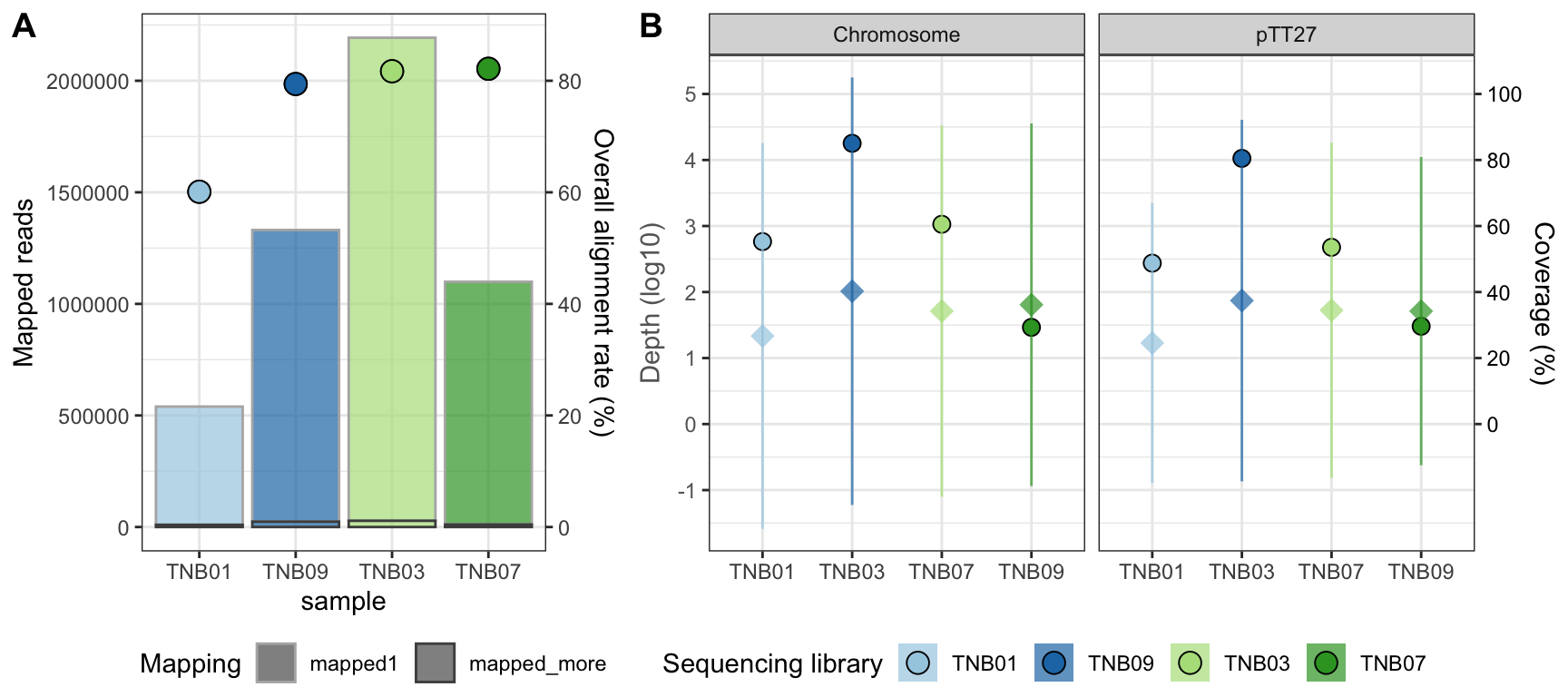
Figure 1. TnSeq libraries mapping statistics. (A) Reference sequence depth (diamonds, left axis) and coverage (round points, right axis). Samples corresponding to ppol and wt HB27 strains are colored in blues and greens, respectively. (B) Total number of mapped reads (bars, left axis) and overall alignment rate (points, right axis).

The mapping shows that overall 80% of the reads mapped once within the HB27 chromosome, giving rise to a good coverage of the HB27 genome, with roughly 100x coverage depth and 50% of coverage breadth. However, again, the sample TNB01 corresponding to ppol (Mother) is clearly different, with less reads and lower mapping rate.

Mapping coverage in HB27 genome

Let’s look in more detail the mapping per base pair, analyzed with Bedtools 2.30.0.

Show code
#load data
coverage <- fread("01_bowtie2/bedtools_output/TNB01_dd_cov_fw.tsv.gz",  header=FALSE, select=c(4,7,8))
coverage <- cbind(coverage, fread("01_bowtie2/bedtools_output/TNB01_dd_cov_rv.tsv.gz",  header=FALSE,select=8),"TNB01")

coverage <- rbind(coverage, cbind( fread("01_bowtie2/bedtools_output/TNB09_dd_cov_fw.tsv.gz",  header=FALSE,select=c(4,7,8)),fread("01_bowtie2/bedtools_output/TNB09_dd_cov_rv.tsv.gz",  header=FALSE,select=8),"TNB09"))

coverage <- rbind(coverage, cbind( fread("01_bowtie2/bedtools_output/TNB03_dd_cov_fw.tsv.gz",  header=FALSE,select=c(4,7,8)),fread("01_bowtie2/bedtools_output/TNB03_dd_cov_rv.tsv.gz",  header=FALSE,select=8),"TNB03"))

coverage <- rbind(coverage, cbind( fread("01_bowtie2/bedtools_output/TNB07_dd_cov_fw.tsv.gz",  header=FALSE,select=c(4,7,8)),fread("01_bowtie2/bedtools_output/TNB07_dd_cov_rv.tsv.gz",  header=FALSE,select=8),"TNB07"))

names(coverage) <- c("Chain","Position","Pos","Neg","Sample")
coverage$Chain <- as.factor(coverage$Chain)
coverage$Sample <- factor(coverage$Sample, levels=c("TNB01","TNB09","TNB03","TNB07"))

#code for circos plot modified from https://www.royfrancis.com/beautiful-circos-plots-in-r/
#coverage for circos processed in external script "scripts/circos.R"
load("scripts/cov_chr.Rdata")

#circos plot
circos.clear()
col_text <- "grey40"
circos.par("track.height"=0.8, gap.degree=0, cell.padding=c(0, 0, 0, 0))
circos.initialize(factors=c("AE017221.1"), 
                  xlim=matrix(c(0, 1894877), ncol=2))

circos.track(ylim=c(0, 1), panel.fun=function(x, y) {
  chr=CELL_META$sector.index
  xlim=CELL_META$xlim
  ylim=CELL_META$ylim
  circos.text(mean(xlim), mean(ylim), chr, cex=0.6, col=col_text, 
              facing="bending.inside", niceFacing=TRUE)
}, bg.col="grey90", bg.border=F, track.height=0.06)

brk <- c(0, 0.25,0.5,0.75, 1, 1.25,1.5, 1.75,2, 2.5, 3)*10^6
circos.track(track.index = get.current.track.index(), panel.fun=function(x, y) {
  circos.axis(h="top", major.at=brk, labels=round(brk/10^6, 2), labels.cex=0.6, 
              col=col_text, labels.col=col_text, lwd=0.7, labels.facing="clockwise")
}, bg.border=F)

#cov tracks

circos.track(factors=cov_chr[[1]]$X1, x=cov_chr[[1]]$X2, y=log10(cov_chr[[1]]$X4+1), panel.fun=function(x, y) {
  circos.lines(x, y, col=my.cols[1], lwd=1)
}, ylim=range(log10(cov_chr[[1]]$X4+1)), track.height=0.1, bg.border=F)


circos.track(factors=cov_chr[[2]]$X1, x=cov_chr[[2]]$X2, y=log10(cov_chr[[2]]$X4+1), panel.fun=function(x, y) {
  circos.lines(x, y, col=my.cols[2], lwd=1)
}, ylim=range(log10(cov_chr[[2]]$X4+1)), track.height=0.08, bg.border=F)

circos.track(factors=cov_chr[[3]]$X1, x=cov_chr[[3]]$X2, y=log10(cov_chr[[3]]$X4+1), panel.fun=function(x, y) {
  circos.lines(x, y, col=my.cols[3], lwd=1)
}, ylim=range(log10(cov_chr[[3]]$X4+1)), track.height=0.08, bg.border=F)


circos.track(factors=cov_chr[[4]]$X1, x=cov_chr[[4]]$X2, y=log10(cov_chr[[4]]$X4+1), panel.fun=function(x, y) {
  circos.lines(x, y, col=my.cols[4], lwd=1)
}, ylim=range(log10(cov_chr[[4]]$X4+1)), track.height=0.08, bg.border=F)

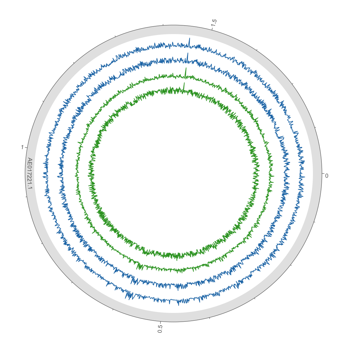
Figure 2. HB27 wt (green) and Ppol (blue) TnSeq libraries mapping in HB27 chromosome. Coverage is represented the mean cov per 1 kb widows in log10 scale. Outer circle scale in Mb.
Show code
#coverage for circos processed in external script "scripts/circos.R"
load("scripts/cov_pTT27.Rdata")


#pTT27 circos plot
circos.clear()
col_text <- "grey40"
circos.par("track.height"=0.8, gap.degree=0, cell.padding=c(0, 0, 0, 0))
circos.initialize(factors=c("AE017222.1"), 
                  xlim=matrix(c(0, 232605), ncol=2))

circos.track(ylim=c(0, 1), panel.fun=function(x, y) {
  chr=CELL_META$sector.index
  xlim=CELL_META$xlim
  ylim=CELL_META$ylim
  circos.text(mean(xlim), mean(ylim), chr, cex=0.6, col=col_text, 
              facing="bending.inside", niceFacing=TRUE)
}, bg.col="grey90", bg.border=F, track.height=0.09)

brk <- c(0, 0.05, 0.1, 0.15, 0.2, 0.25, 0.3)*10^6
circos.track(track.index = get.current.track.index(), panel.fun=function(x, y) {
  circos.axis(h="top", major.at=brk, labels=round(brk/10^6, 2), labels.cex=0.6, 
              col=col_text, labels.col=col_text, lwd=0.7, labels.facing="clockwise")
}, bg.border=F)

#cov tracks
circos.track(factors=cov[[1]]$X1, x=cov[[1]]$X2, y=log10(cov[[1]]$X4+1), panel.fun=function(x, y) {
  circos.lines(x, y, col=my.cols[1], lwd=1)
}, ylim=range(log10(cov[[1]]$X4+1)), track.height=0.08, bg.border=F)

circos.track(factors=cov[[2]]$X1, x=cov[[2]]$X2, y=log10(cov[[2]]$X4+1), panel.fun=function(x, y) {
  circos.lines(x, y, col=my.cols[2], lwd=1)
}, ylim=range(log10(cov[[2]]$X4+1)), track.height=0.08, bg.border=F)

circos.track(factors=cov[[3]]$X1, x=cov[[3]]$X2, y=log10(cov[[3]]$X4+1), panel.fun=function(x, y) {
  circos.lines(x, y, col=my.cols[3], lwd=1)
}, ylim=range(log10(cov[[3]]$X4+1)), track.height=0.08, bg.border=F)


circos.track(factors=cov[[4]]$X1, x=cov[[4]]$X2, y=log10(cov[[4]]$X4+1), panel.fun=function(x, y) {
  circos.lines(x, y, col=my.cols[4], lwd=1)
}, ylim=range(log10(cov[[4]]$X4+1)), track.height=0.08, bg.border=F)

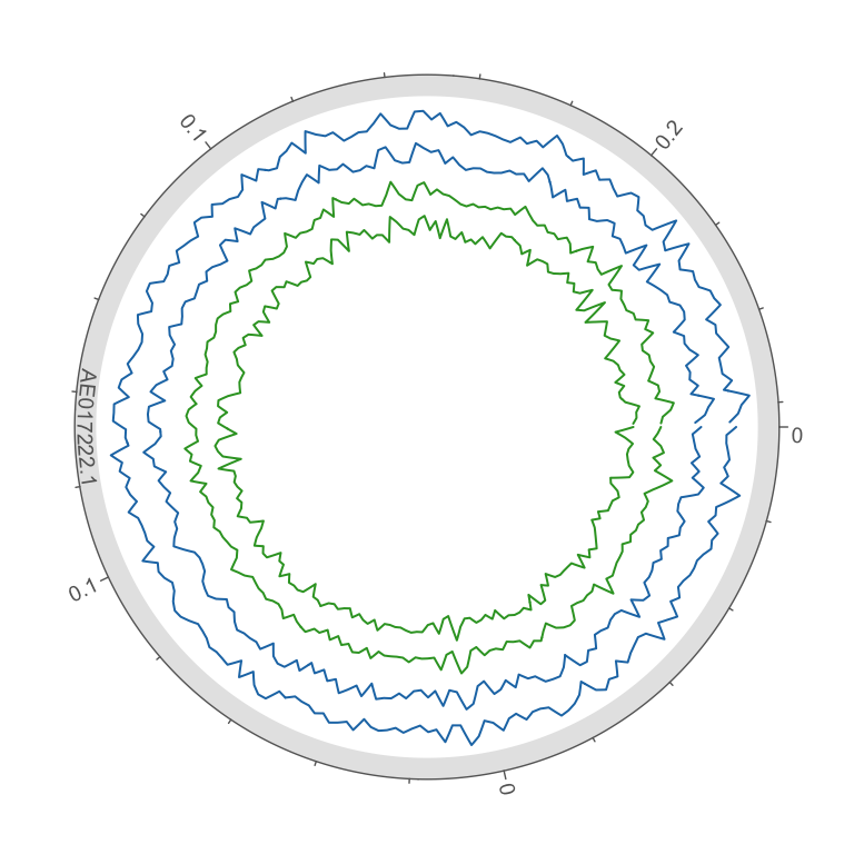
Figure 3. HB27 wt (green) and Ppol (blue) TnSeq libraries mapping in pTT27 plasmid. Coverage is represented the mean cov per 1 kb widows in log10 scale. Outer circle scale in Mb.

The above plots represent mean coverage per 1000 bp windows, full plots are in the folder bamdash and can be accessed with the following links, as interactive plots and SVG images.

Table 2. BAMdash coverage plots
Sample Chromosome pTT27 plasmid
HB27 Report - SVG Report - SVG
HB27_rep Report - SVG Report - SVG
ppol Report - SVG Report - SVG
ppol_rep Report - SVG Report - SVG

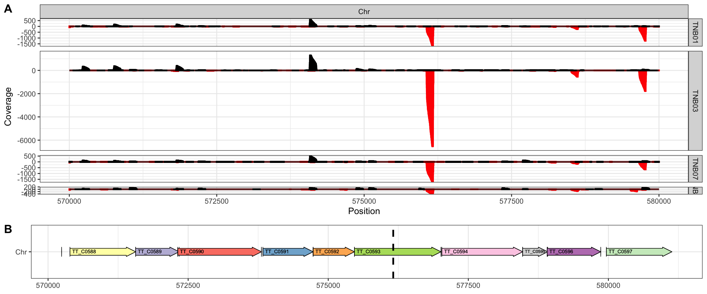
The two replicates have a smaller range than the primary samples (mother and daughter), but we can still recognize two regions with a very high frequency of insertions in the reverse strand, located at positions 576,160 and 1,457,335 of the chromosome and almost overlapping in the four samples.

We have now decided to investigate these regions in more detail. The first hotspot corresponds to gene TT_C0593 (Figure 3), which encodes a 5-carboxymethyl-2-hydroxymuconate semialdehyde dehydrogenase, an oxidoreductase involved in tyrosine metabolism that may be dispensable in rich media. This target region corresponds to a GC track, the preferred sequence for Tn5 (Green et al. 2012). However, as the coverage indicates multiple nearby integration sites, the high integration rate within TT_C0593 may indicate that this gene is not required rather than a transposase artifact.

Show code
cov <- ggplot(coverage[coverage$Position > 570000 & coverage$Position < 580000]) +  geom_bar(aes(x=Position,y=Neg * -1),color="red", stat="identity", linewidth=1) +
  geom_bar(aes(x=Position,y=Pos),color="black", stat="identity",linewidth=1) +
  facet_grid(Sample~Chain, space = "free", scales="free_y")+theme_bw()+ylab("Coverage")

coding <- read.table("00_raw/refs/GCA_000008125.1.gtf",sep="\t",header=FALSE)

genes <- ggplot(coding[coding$V4 > 570000 & coding$V4 < 579000,], aes(xmin = V4, xmax = V5, y = V1, fill = substr(V9,9,16), label=substr(V9,9,16))) +
  geom_gene_arrow() +
  geom_gene_label(align = "left")+
  theme_bw() +
  geom_vline(xintercept =576160, linetype="dashed",linewidth=1) +
  scale_fill_brewer(palette = "Set3") +theme(legend.position="none",plot.margin=margin(0,1,0,0.75,unit = "cm")) + ylab("") + scale_y_discrete(labels="Chr") + scale_x_continuous(breaks = seq(570000, 580000, 2500))

ggarrange(cov, genes, 
          labels = c("A", "B"), ncol=1,heights=c(3,1)
         )

Figure 4. TnSeq insertion hotspot (A) Detailed coverage (linear scale) in the region 570000-580000 of HB27 chromosome in each sample, Ppol (TNB01), Ppol_rep (TNB09), HB27 (TNB03) and HB27_rep (TNB07). (B) Annotated features in the detailed region. The vertical dashed line indicated the position of the highest coverage.

The second and more strong hotspot (Figure 5) is located in an intergenic region between locus TT_C1532 (glucosamine-fructose-6-phosphate aminotransferase) and TT_C1533 (S-layer protein). The sequence in this point appears to be more diverse but also contains GC traces. This hostpot is likely consequence of the use of S-layer protein promoter in front of the kanamycin resistance gene used for the transposition selection. Moreover, since we will normalize the counts per gene based on the mapped reads in the coding regions (see below), this promiscuous site will not affect our analysis.

Show code
cov <- ggplot(coverage[coverage$Position > 1447000 & coverage$Position < 1459500]) +  geom_bar(aes(x=Position,y=Neg * -1),color="red", stat="identity", linewidth=1) +
  geom_bar(aes(x=Position,y=Pos),color="black", stat="identity",linewidth=1) +
  facet_grid(Sample~Chain, space = "free", scales="free_y")+theme_bw()+ylab("Coverage")

genes <- ggplot(coding[coding$V4 > 1445000 & coding$V4 < 1458000,], aes(xmin = V4, xmax = V5, y = V1, fill = substr(V9,9,16), label=substr(V9,9,16))) +
  geom_gene_arrow() +
  geom_gene_label(align = "left")+
  theme_bw() +
  geom_vline(xintercept =1457335, linetype="dashed",linewidth=1) +
  scale_fill_brewer(palette = "Set3") +theme(legend.position="none",plot.margin=margin(0,0.8,0,0,unit = "cm")) + ylab("") + scale_y_discrete(labels="Chr") + scale_x_continuous(breaks = seq(1444000, 1457000, 4000))

ggarrange(cov, genes, 
          labels = c("A", "B"), ncol=1,heights=c(3,1)
         )

Figure 5. TnSeq insertion hotspot (A) Detailed coverage in the region 1445000-1458000 of HB27 chromosome in each sequencing library: Ppol (TNB01), Ppol_rep (TNB09), HB27 (TNB03) and HB27_rep (TNB07). (B) Annotated features in the detailed region. The vertical dashed line indicated the position of the highest coverage.

Tn5 transposon insertions per gene and Z-score

Count integration events counts per gene and Z-score calculation

Now we are going to transform the mapped reads into hits per gene, to obtain a normalized insertion score, by the following steps:

  1. We only consider insertions within the 10-90% interval of each gene, because insertions landing in the flanking sections of genes might give rise to truncated of chimeric proteins partially functional. The counts of Tn insertions will be obtained from the read mapping coordinates, considering the alignment start and the strand, after conversion of the BAM file to a tabulated format (BED).

  2. We will normalize by the total number of mapped reads within the coding regions (80% central).

  3. We will obtain a ratio of observed to expected Tn insertions.

  4. We will make a log2-transformation in pseudocounts \(log_2(x+1)\) to avoid negative scores.

  5. Finally, we will scale the data to favor sample comparison, using the R function scale() to obtain a final Z-score.

Thus, our score will be obtained with the following formula:

\[ Score = log_2 \left( \frac{count}{\text{sample mapped reads} * \frac{\text{gen length} }{\text{genome length}}} +1 \right) \]

And the final Z-score will be:

\[ \textbf{Z}{-}\textbf{Score} = \frac{Score - mean(Score)}{SD(Score)} \]

In the following plots you can see the distribution of Z-scores between samples.

Show code
cd ~/data/TnSeq_thermus
bedtools bamtobed -i 01_bowtie2/mapping_TNB03_dd_sorted.bam > 01_bowtie2/mapping_TNB03_dd_sorted.bed

bedtools bamtobed -i 01_bowtie2/mapping_TNB01_dd_sorted.bam > 01_bowtie2/mapping_TNB01_dd_sorted.bed

bedtools bamtobed -i 01_bowtie2/mapping_TNB07_dd_sorted.bam > 01_bowtie2/mapping_TNB07_dd_sorted.bed

bedtools bamtobed -i 01_bowtie2/mapping_TNB09_dd_sorted.bam > 01_bowtie2/mapping_TNB09_dd_sorted.bed
Show code
#gene table formatted with 80% central gene
HB27_genome <- read.table("00_raw/refs/GCA_000008125.1.gtf",sep="\t",header=FALSE)
HB27_genome$Chr <- "AE017221.1"
HB27_genome$Chr[8088:nrow(coding)] <- "AE017222.1"
HB27_genome$V9 <-  substr(HB27_genome$V9,9,16)

#correct TT_C0145 coordinates and remove TT_C0146
HB27_genome$stop[HB27_genome$Genes=="TT_C0145" & HB27_genome$V3=="gene"] <- HB27_genome$stop[HB27_genome$Genes=="TT_C0146" & HB27_genome$V3=="gene"]
HB27_genome[-as.numeric(rownames(HB27_genome[HB27_genome$Genes=="TT_C0146",])),]
 [1] V1  V2  V3  V4  V5  V6  V7  V8  V9  Chr
<0 rows> (or 0-length row.names)
Show code
#select "gene" feature for mapping
HB27_genome80 <- HB27_genome[HB27_genome$V3=="gene",]

#subset the 10-90% gene interval and reshape table
HB27_genome80 <- data.frame(HB27_genome80[,c(9,1,4,5,7)])
colnames(HB27_genome80) <- c("GeneID","Chr","Start","End","Strand")
HB27_genome80$Start <- HB27_genome80$Start + (HB27_genome80$End - HB27_genome80$Start) * 0.1
HB27_genome80$End <- HB27_genome80$End - (HB27_genome80$End - HB27_genome80$Start) * 0.1
HB27_genome80 <- HB27_genome80[,c(1,2,5,3,4)]

#load BED files
samples <- c("Ppol_1"="TNB01", "Ppol_2"="TNB09","HB27_1"="TNB03", "HB27_2"="TNB07")

data <- list()
insertion_table <- list()
scores_table <- list()
#prepare HB27_genome80 for foverlaps()
names(HB27_genome80) <- c("Gene","Chr","Str","start","end") 
HB27_genome80 <- as.data.table(HB27_genome80)
setkey(HB27_genome80, start, end) #keyed

#match read mapping start with genes coordinates to obtain insertion sites per gene
for (i in 1:4){
  data[[i]] <- fread(input = paste0("01_bowtie2/mapping_",samples[i],"_dd_sorted.bed"))
  #filter by alignment quality
  data[[i]] <- data[[i]][data[[i]]$V5 > 5]
    data[[i]] <- data[[i]][,c(1,6,2,3)]
    names(data[[i]]) <- c("Mapped_Chr","Strand","start","end")
    insertion_table[[i]] <- foverlaps(as.data.table(data[[i]]),HB27_genome80,type="within",nomatch = 0,mult="all")
    insertion_table[[i]] <- subset(insertion_table[[i]], Chr==Mapped_Chr)
    insertion_table[[i]] <- insertion_table[[i]][,-9]
    scores_table[[i]] <- as.data.frame(table(insertion_table[[i]]$Gene))
    names(scores_table[[i]]) <- c("Gene","Counts")
    scores_table[[i]] <- merge(as.data.frame(HB27_genome80),scores_table[[i]], all.x=TRUE)
    scores_table[[i]]$Counts <- ifelse(is.na(scores_table[[i]]$Counts),0,scores_table[[i]]$Counts)
    scores_table[[i]]$score <- log2((scores_table[[i]]$Counts / (nrow(insertion_table[[i]])* (scores_table[[i]]$end-scores_table[[i]]$start)/2127482)) +1 )
  }

tnseq <- merge(scores_table[[1]],scores_table[[2]], by=c("Gene","Chr","Str","start","end"),all=TRUE)
tnseq <- merge(tnseq,scores_table[[3]], by=c("Gene","Chr","Str","start","end"),all=TRUE)
tnseq <- merge(tnseq,scores_table[[4]],by=c("Gene","Chr","Str","start","end"),all=TRUE)
names(tnseq) <- c("Gene","Chr","Str","Start80","End80","Counts_Ppol_1","Zscore_Counts_Ppol_1","Counts_Ppol_2","Zscore_Ppol_2","Counts_HB27_1","Zscore_HB27_1","Counts_HB27_2","Zscore_HB27_2")
#write.table(tnseq,"tnseq_dd_counts_scores_all.csv",quote=FALSE,sep=";",row.names = FALSE)
 

scores <- as.data.frame(scale(tnseq[,c(7,9,11,13)]))
names(scores) <- c("Ppol_1","Ppol_2","HB27_1","HB27_2")
row.names(scores) <- tnseq$Gene
#write.table(scores,"scores80_11nov2024.csv",row.names = TRUE,sep=";")


#plot distribution
box <- ggplot(stack(scores), aes(x=ind, y=values)) + xlab("") + 
  ylab("Score")+
  geom_boxplot(outlier.shape=8,outlier.size=3,aes(color=ind,fill=ind,alpha=0.8),
               linewidth = 1)+theme_linedraw()+geom_jitter(alpha=0.1,aes(color=ind)) +
 # geom_point(data=q,aes(x=ind,y=values,fill=ind),shape=23,size=4) +
  theme(axis.text.x = element_text(face="bold", vjust=1))+
  theme(legend.position = "none") + scale_color_brewer(palette="Paired")+
  scale_fill_brewer(palette="Paired")

#correlation
wt <- ggplot(data = scores, aes(x=HB27_1,y=HB27_2))+geom_point(size=3,alpha=0.6, color=my.cols[4]) +  theme_linedraw() + ylim(-2,7) +
  xlab("HB27_1") + ylab("HB27_2") + stat_poly_line(color=my.cols[4],fill=my.cols[4]) +
  stat_poly_eq(use_label(c("adj.R2", "p"))) 


ppol <- ggplot(data = scores, aes(x=Ppol_1,y=Ppol_2))+geom_point(size=3,alpha=0.6, color=my.cols[2])  + theme_linedraw() + ylim(-2,7) +
  xlab("Ppol_1") + ylab("Ppol_2") +  stat_poly_line(color=my.cols[2],fill=my.cols[2]) +
  stat_poly_eq(use_label(c("adj.R2", "p"))) 

ggarrange(box, ppol, wt,
          labels = c("A", "B","C"), ncol=1
         )

Figure 6. Tn insertion Z-scores per gene. (A) Boxplot of gene Z-scores per sample. (B & C) Correlation of Z-scores per gene between sample replicates.

As we can see, the correlation between the two PPOL samples is only moderate, in line with the QC and mapping results. To analize this in more detail and compare the four samples, we used a PCA plot. As shown in Figure 7 below, the first variable is responsible for >80% of the data variability, with all samples being very similar in this direction. A second variable is responsible for ~10% of the data diversity, with half of this divergence attributable to sample Ppol_2 (TNB09). Interestingly, samples TNB01, TNB03 and TNB07 are quite similar, although sample TNB01 contains significantly fewer reads, suggesting that the sequencing library does not strongly influence our results.

Show code
tnseq.pca <- prcomp(na.omit(scores)[,1:4], 
                   center = TRUE, 
                   scale = TRUE) 
fviz_pca_biplot(tnseq.pca,col.var=rownames(tnseq.pca[[2]]),col.ind="grey90", label="var",labelsize=5,labelface="bold")+ylim(-4,4)+xlim(-2.5,9)+scale_color_brewer(palette="Paired")+theme_pubclean()+theme(legend.position="none")

Figure 7. Samples PCA plot. Note that only complete cases (genes with at least one Tn5 insertion in all samples) can be used.

In order to analyze in detail the difference between samples, we construct also a plot in which we plot the Z-scores for all genes in all samples.

Show code
scores$mean <- apply(scores, 1, mean,na.rm=TRUE)
kk <- cbind(tnseq$Gene,scores$mean,stack(scores))
dis <- ggplot(data=kk) +
  geom_point(aes(x=reorder(`tnseq$Gene`,`scores$mean`,decreasing=TRUE),y=values,color=ind), alpha=0.7)+
  theme_classic() +
  scale_x_discrete(expand = c(0.01, 0)) + 
  theme(axis.text.x = element_blank(),axis.text.y=element_text(size=12,face="bold")) +
  ylab("Z-Score") + xlab("Gene") +
  scale_color_brewer(palette="Paired") + theme(legend.position = c(0.9, 0.7)) +
  labs(color="")
#ggsave("fig2a.pdf",dis,width=6,height=3)
ggplotly(dis)

Figure 8. Comparison of Tn insertion Z-scores per gene. Values were sorted by the average of all samples. This is an interactive plot: Put your mouse pointer over any point and you will see a pop-up label with the Z-score and the Gene info.

It is striking that we do not see a step that marks the boundary between the group of non-essential genes, which are expected to have a higher score, and the essential genes with very low or no Tn5 insertions and thus a low score.

Summary stats

In the following table you can find a summary of the main raw insertion stats. The average number of insertions within the 80% central portion of the gene was around 1.8x10^5, with roughly 4.7 x10^4 unique insertion sites, that is an average of 1 unique insertion site per 44.8 bp.

Show code
kk <- cbind(insertion_table[[1]], "HB27_1")
kk <- rbind(kk,cbind(insertion_table[[2]], "HB27_2"))
kk <- rbind(kk,cbind(insertion_table[[3]], "Ppol_1"))
kk <- rbind(kk,cbind(insertion_table[[4]], "Ppol_2"))
#unique insertions per sample and per strand
unique_insertions <- aggregate(data=kk, i.start ~ Strand+V2, function(x) length(unique(x)))
#unique insertions total per sample
unique_insertions <- aggregate(unique_insertions,unique_insertions$i.start~unique_insertions$V2,sum)
#all
resumen <- cbind(fastp[,c(1,4)],as.vector(table(kk$V2)),unique_insertions[,2])
#normalized & ratio
resumen$normalized <- resumen[,4]/resumen[,2]
resumen[,2] <- resumen[,2] * 1000000
resumen$ratio <- paste(as.character(round(resumen[,4]*100/resumen[,3],1)),"%")
resumen[5,] <- c("Mean",apply(resumen[,2:5],2,mean),paste(as.character(round(mean(resumen[,4]*100/resumen[,3]),1)),"%"))
resumen[,2] <- as.numeric(resumen[,2])
resumen[,3] <- as.numeric(resumen[,3])
resumen[,4] <- as.numeric(resumen[,4])
resumen[,5] <- as.numeric(resumen[,5])

as.data.frame(format(resumen[c(1,4,3,2,5),c(1:4,6,5)], scientific = TRUE, digits = 3)) %>% 
kbl(align = "c", row.names = FALSE,col.names= c("Sample","Filtered Reads","Insertions 80% ORF","Unique insertions 80% ORF","Ratio unique","Normalized Unique insertions per M Reads"), caption = "Table 3. Summary of TnSeq statistics") %>%
    kable_styling(bootstrap_options = "striped", full_width = F, position = "center") %>%
    column_spec(1, bold = T, italic=T, color=c(my.cols,"grey30"))
Table 3. Summary of TnSeq statistics
Sample Filtered Reads Insertions 80% ORF Unique insertions 80% ORF Ratio unique Normalized Unique insertions per M Reads
Ppol_1 9.00e+05 1.05e+05 3.69e+04 35.2 % 4.10e+04
Ppol_2 1.70e+06 1.64e+05 4.39e+04 26.7 % 2.58e+04
HB27_2 1.30e+06 2.88e+05 7.14e+04 24.8 % 5.49e+04
HB27_1 2.70e+06 1.56e+05 3.77e+04 24.1 % 1.40e+04
Mean 1.65e+06 1.78e+05 4.75e+04 27.7 % 3.39e+04

Insertions in key genes

We now decided to check some genes, expected to be essential, and see their score and the number and location of the insertions in each sample.

Show code
#read Table
LH <- read_xlsx("DNAprocessestoGraph.xlsx",sheet=1)
LH <- LH[grep("TT_C",LH$Genes),]
coding$Genes <- substr(coding$V9,9,16)
tmp <- coding[coding$V3=="CDS"|coding$V3=="transcript",c(1,10,4,5)]
tmp <- tmp[tmp$Genes %in% LH$Genes,]


kk$Strand <- as.logical(kk$Strand=="+")
keygenes <- list()

keygenes <- lapply(1:nrow(tmp), FUN = function(i) {
  tmp2 <- tmp[c(i,i,i,i),]
  tmp2$V1 <- names(samples)
  keygenes[[i]] <- ggplot(tmp2, aes(xmin = V4, xmax = V5, y = forcats::fct_rev(V1),  label=Genes)) +
    geom_gene_arrow(fill="grey90",arrowhead_width = grid::unit(8, "pt"), arrowhead_height = grid::unit(16, "pt"), arrow_body_height = grid::unit(11, "pt")) +
    geom_feature(data = kk[kk$Gene %in% tmp2[,2],], aes(x = i.start, y = V2, color=Strand),feature_height = unit(8, "mm")  ) + scale_color_discrete(name = "Strand", labels = c("Reverse", "Forward")) + 
    geom_gene_label(fontface="bold",align="left",grow=TRUE,height = grid::unit(12, "pt"))+
    theme_bw() + theme(legend.position="none") +
    theme(axis.text.x = element_text(angle = 45, vjust = 1, hjust=1),text=element_text(face="bold"))+
    ylab("") + xlab("")+ labs(subtitle=paste("Mean Z-score:",round(scores$mean[row.names(scores)==tmp$Genes[i]],2)))
})
do.call("grid.arrange", c(keygenes, ncol = 3))

Figure 9. Tn insertions in key HB27 genes in forward (blue) and reverse (pink) strands. Only insertions between 10-90% central gene interval considered for Z-score calculation are displayed.
Show code
sessionInfo()
R version 4.4.1 (2024-06-14)
Platform: x86_64-apple-darwin20
Running under: macOS Sonoma 14.6.1

Matrix products: default
BLAS:   /Library/Frameworks/R.framework/Versions/4.4-x86_64/Resources/lib/libRblas.0.dylib 
LAPACK: /Library/Frameworks/R.framework/Versions/4.4-x86_64/Resources/lib/libRlapack.dylib;  LAPACK version 3.12.0

locale:
[1] en_US.UTF-8/en_US.UTF-8/en_US.UTF-8/C/en_US.UTF-8/en_US.UTF-8

time zone: Europe/Madrid
tzcode source: internal

attached base packages:
[1] stats     graphics  grDevices utils     datasets  methods   base     

other attached packages:
 [1] RColorBrewer_1.1-3  factoextra_1.0.7    circlize_0.4.16    
 [4] gridExtra_2.3       readxl_1.4.5        ggpmisc_0.6.1      
 [7] ggpp_0.5.8-1        plotly_4.10.4       details_0.4.0      
[10] ggpubr_0.6.0        lubridate_1.9.4     forcats_1.0.0      
[13] stringr_1.5.1       purrr_1.0.4         readr_2.1.5        
[16] tidyr_1.3.1         tibble_3.2.1        tidyverse_2.0.0    
[19] dplyr_1.1.4         Rsubread_2.20.0     gggenes_0.5.1      
[22] kableExtra_1.4.0    data.table_1.17.0   ggplot2_3.5.1      
[25] formatR_1.14        knitr_1.50          BiocManager_1.30.25

loaded via a namespace (and not attached):
 [1] tidyselect_1.2.1    viridisLite_0.4.2   farver_2.1.2       
 [4] R.utils_2.13.0      fastmap_1.2.0       lazyeval_0.2.2     
 [7] digest_0.6.37       timechange_0.3.0    lifecycle_1.0.4    
[10] survival_3.8-3      magrittr_2.0.3      compiler_4.4.1     
[13] rlang_1.1.5         tools_4.4.1         yaml_2.3.10        
[16] ggsignif_0.6.4      labeling_0.4.3      htmlwidgets_1.6.4  
[19] xml2_1.3.8          abind_1.4-8         withr_3.0.2        
[22] R.oo_1.27.0         desc_1.4.3          grid_4.4.1         
[25] colorspace_2.1-1    scales_1.3.0        MASS_7.3-65        
[28] cli_3.6.4           rmarkdown_2.29      generics_0.1.3     
[31] rstudioapi_0.17.1   httr_1.4.7          tzdb_0.4.0         
[34] polynom_1.4-1       splines_4.4.1       cellranger_1.1.0   
[37] vctrs_0.6.5         Matrix_1.7-3        jsonlite_1.9.1     
[40] carData_3.0-5       SparseM_1.84-2      confintr_1.0.2     
[43] car_3.1-3           hms_1.1.3           ggrepel_0.9.6      
[46] rstatix_0.7.2       Formula_1.2-5       crosstalk_1.2.1    
[49] systemfonts_1.2.1   clipr_0.8.0         glue_1.8.0         
[52] cowplot_1.1.3       stringi_1.8.4       gtable_0.3.6       
[55] shape_1.4.6.1       munsell_0.5.1       pillar_1.10.1      
[58] htmltools_0.5.8.1   quantreg_6.1        ggfittext_0.10.2   
[61] R6_2.6.1            evaluate_1.0.3      lattice_0.22-6     
[64] R.methodsS3_1.8.2   png_0.1-8           backports_1.5.0    
[67] broom_1.0.7         MatrixModels_0.5-3  Rcpp_1.0.14        
[70] svglite_2.1.3       xfun_0.51           pkgconfig_2.0.3    
[73] GlobalOptions_0.1.2
Back to top

References

Chen, Shifu, Yanqing Zhou, Yaru Chen, and Jia Gu. 2018. “fastp: an ultra-fast all-in-one FASTQ preprocessor.” Bioinformatics (Oxford, England) 34 (17): i884–90. https://doi.org/10.1093/bioinformatics/bty560.
Green, Brian, Christiane Bouchier, Cécile Fairhead, Nancy L. Craig, and Brendan P. Cormack. 2012. “Insertion Site Preference of Mu, Tn5, and Tn7 Transposons.” Mobile DNA 3 (1): 3. https://doi.org/10.1186/1759-8753-3-3.

Footnotes

  1. For Tn insertions purposes, we merged the TT_C0145 and TT_C0146 genes, based on (unpublished) evidence from Mencía lab.↩︎

MRR, 2024